Exploring spaces and maps
An encoding can come from a filtration of data or from a module described directly by geometric regions. In either case, which space belongs to a parameter you care about, and what happens to its vectors when you move to another parameter? TamerOp lets you compute these spaces and maps, examine their matrices, and connect the answer to a picture of the finite representation.
This guide starts with an EncodingResult and follows those choices. You need the meaning of a space and structure map, but need not work through another construction lesson first. To construct your starting object, start from a filtration or define a module by regions. That guide uses the same kinds of queries for both routes. The square notebook develops the mathematics through a complete worked example; here the emphasis is on choosing queries you can reuse with your own encoding. If you already have a finite PModule, you can begin with finite-label queries and omit parameter lookup.
Start from a recognizable object
The following setup makes the square-supported module: a one-dimensional space on the closed square [0,2] × [0,2], zero elsewhere, with identity maps between comparable interior parameters. Its coefficients are rational. Replace this setup with your own enc when exploring another object.
import TamerOp as OP
import TamerOp.Advanced as OA
import TamerOp.CoreModules: QQField

options = OA.EncodingOptions(; backend=:pl_backend,
    poset_kind=:signature, field=QQField())
enc = OP.encode([OA.BoxUpset([0, 0])], [OA.BoxDownset([2, 2])],
    reshape(OP.QQ[1], 1, 1), options);
OP provides the main workflow. OA gives access to the more detailed queries used below, including finite-label lookup and presentation inspection. The two indicator regions and their coefficient describe the input; encode returns the finite representation. See indicator presentations for the construction, including what the active rows and columns mean.
An encoding keeps the finite poset, the assignment from parameters to its labels, and the encoded module together. Ask what is retained before choosing what to compute:
OP.describe(enc)
OP.provenance(enc)
The summary describes stored information; provenance records the construction and its conventions, including the field. This square constructor already computes its module. Some ingestion workflows instead return a lazy result: enough information to compute spaces and maps when requested. Displaying such a result leaves that work deferred.
| What you need | Query | What it asks for |
|---|---|---|
| Finite labels and their order | OP.encoding_poset(enc) | The retained poset |
| Assignment from parameters to labels | OP.encoding_map(enc) | The retained classifier |
| Every stalk dimension | OP.dimensions(enc) | A dimension vector, computing it if needed |
| Spaces with their structure maps | OP.encoding_module(enc) | The finite module, materializing it if needed |
| A retained indicator presentation | OP.encoding_presentation(enc) | The finite fringe, or nothing if absent |
Dimension queries can do mathematical work even though they return only integers. Having the dimensions does not imply that lazy structure maps have been computed. The deferred-computation guide explains reuse and costs across ingestion, algebra and geometry.
Find a parameter's space
Keep the poset and its parameter assignment available, then ask for dimensions:
P = OP.encoding_poset(enc)
classifier = OP.encoding_map(enc)
dims = OP.dimensions(enc)
dims[q] is the dimension at finite label q. These integers are labels in the returned poset, not parameter coordinates or ranks in a sorted list. The signature encoder used here returns four labels; the nine-region picture in finite encodings is another valid description of the same square. Obtain labels from this result instead of assuming their numbers.
x = (1//2, 1//2)
qx = OA.locate(classifier, x)
(label=qx, dimension=dims[qx])
The dimension is 1. The expression 1//2 supplies the exact rational one-half. A parameter first chooses a label; that label chooses a space. This is also how the picture and the algebra refer to the same object.
For classifiers that do not represent the whole parameter domain, locate can return 0. Check for that sentinel before indexing a dimension vector:
z = (3, 1)
qz = OA.locate(classifier, z)
z_dimension = qz == 0 ? nothing : dims[qz]
Here qz is a represented label and z_dimension is 0: the point is outside the square's support, but its zero space is part of the encoding. An unrepresented point would instead give nothing in this example code. The distinction is useful for encodings whose classifier covers only part of the parameter domain; missing information does not determine a zero space.
If your starting object is already a finite module M, use OA.dim_at(M, q) for a single stalk dimension. OP.dimensions(M) returns a summary with a .stalks vector; OP.dimensions(enc) returns that vector directly.
Ask how vectors continue
A matrix answers a different question from a dimension. Its columns correspond to the source space's coordinates, and its rows to the target's. Materialize the finite module when you need these maps:
M = OP.encoding_module(enc)
y = (3//2, 3//2)
qy = OA.locate(classifier, y)
A = OA.structure_map(M; source=qx, target=qy)
The answer is the 1 × 1 identity matrix over the rationals: the vector continues unchanged. structure_map takes finite labels. It can compose cover maps when the selected pair is not itself a cover; you need not build a table of all comparable pairs. Returned matrices may share stored data, so treat them as read-only, or copy(A) before editing entries.
Now move beyond the support:
Z = OA.structure_map(M; source=qx, target=qz)
size(Z)
The shape is (0, 1). This is the defined zero map from a one-dimensional space to the zero space. An empty array here has precise mathematical content. Equal labels give the identity on their space, including a 0 × 0 identity for a zero space.
There is an important choice when the question begins with parameters. Finite-label queries know the finite order; they do not check whether the original parameters were comparable. In the square, (1/4,3/2) and (3/2,1/4) have the same label but are incomparable in coordinatewise order. The finite identity at that label is not an ambient structure map between those points. Use a parameter-aware inspection request for this question:
u, v = (1//4, 3//2), (3//2, 1//4)
unordered_view = OA.visual_spec(enc; kind=:module_inspector,
    parameter_pair=(u, v))
unordered = OA.visual_metadata(unordered_view).inspection
(defined=unordered.defined, matrix=unordered.matrix)
The answer is (defined=false, matrix=nothing). A specification is the mathematical content of a view; building it needs no plotting package. The parameter query checks the original order as well as classification. Grid classifiers use their declared axis orientations, rather than assuming every parameter increases in the usual coordinate order.
Keep these outcomes separate when exploring your own object:
| Outcome | Interpretation |
|---|---|
A represented stalk has dimension 0 | Its vector space is zero. |
A defined map has rank 0 | Every source vector maps to zero; the map can have nonempty matrix dimensions. |
| A pair is incomparable or ordered only in reverse | There is no structure map in the requested direction. |
A parameter has classifier label 0 | This encoding does not supply its space or map. |
| A presentation or source representative is absent | The retained result does not include that additional description. |
The last case depends on what was retained, not on whether the selected space is zero. In particular, a coordinate vector in a finite module does not by itself identify a cycle in an input complex.
Connect the answer to a figure
Load CairoMakie for static figures. A single inspection view connects the selected parameters, their finite labels, and the map readout:
import CairoMakie

view_box = ([-1, -1], [5, 5])
map_view = OA.visual_spec(enc; kind=:module_inspector,
    parameter_pair=(x, z), box=view_box)
OP.visualize(map_view)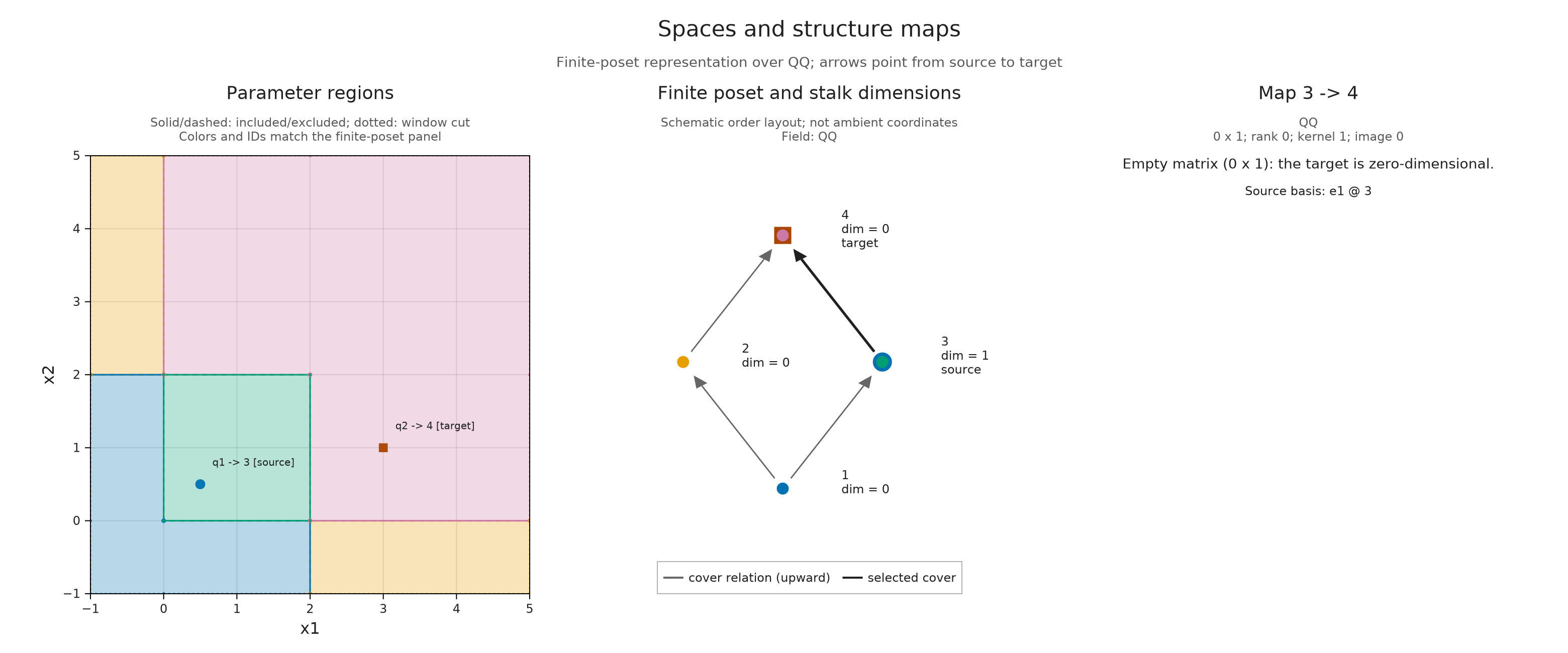
The selected source lies inside the square and the target lies outside its support. The readout reports the 0 × 1 matrix, rank zero and kernel dimension one. Colors and labels connect the parameter plane to the actual finite poset; that poset's layout is schematic.
Select either figure in this guide to open it at full size.
The window makes unbounded regions drawable. It does not restrict the module queried by this inspector. Solid poset arrows are cover relations; a selected comparable non-cover pair receives an additional dashed arrow. The parameter-plane conventions explain included boundaries, window cuts and finite drawing precision.
The same request works without retaining a specification: OP.visualize(enc; kind=:module_inspector, parameter_pair=(x,z), box=view_box). Keep a specification when you want to inspect its data or render the same answer again:
answer = OA.visual_metadata(map_view).inspection
(rank=answer.rank, kernel=answer.kernel_dimension, matrix=answer.matrix)
Choose one selection form per request:
| Question | Selection |
|---|---|
| Space at an original parameter | point=x |
| Map between original parameters | parameter_pair=(x,y) |
| Space at a finite label | vertex=qx |
| Map in the finite model | pair=(qx,qy) |
A PModule has the finite-poset and readout panels without invented geometric coordinates. A supported planar encoding adds its parameter panel. Use OP.available_visuals(enc) to discover its views, or OA.check_visual_request(enc; kind=:module_inspector) to inspect the accepted options and qualitative work. kind=:hasse asks only for the finite order with dimensions; an unselected or stalk-only module inspector also leaves lazy structure maps deferred. A defined pair can materialize them.
Large selected matrices are cropped for display using matrix_limit=(12,12) by default. The specification retains the full matrix; rank and kernel dimension use all its entries. Raising or lowering the display limit changes neither the result nor the cost of constructing it. With RealField, ranks use the field's numerical tolerances; the rational example here is exact.
Look inside a retained presentation
The module's matrix describes a map in its stored coordinate bases. A retained indicator presentation answers an additional question: how do its active coefficient blocks produce those spaces? Start by checking for the witness:
H = OP.encoding_presentation(enc)For this encoding, H is a finite fringe. If the accessor returns nothing, this inspection route is unavailable; it does not reconstruct a presentation from the module. Presentation queries also accept a finite FringeModule directly. The witness must belong to the current poset and field.
To see why counting active generators is insufficient, keep the square's support but give it two active columns in the upper part of the square:
redundant = OP.encode([OA.BoxUpset([0, 0]), OA.BoxUpset([1, 1])],
    [OA.BoxDownset([2, 2])], OP.QQ[1 1], options)
qr = OA.locate(OP.encoding_map(redundant), y)
stalk = OA.presentation_stalk(redundant; vertex=qr)
(rows=OA.active_rows(stalk), columns=OA.active_columns(stalk),
    block=OA.presentation_matrix(stalk),
    dimension=OA.presentation_summary(stalk).dimension)
At y=(3/2,3/2), row 1 and columns 1,2 are active. Their block is [1 1], whose image has dimension one. Two columns supply the same direction. The default query computes the block and its rank, leaving an image basis uncomputed. Request that basis when you want actual vectors in the active downset coordinates:
with_basis = OA.presentation_stalk(redundant; vertex=qr, basis=true)
B = OA.image_basis(with_basis)
size(B)
The shape is (1, 1): one basis vector in one active target coordinate. In general, the basis matrix's row count is the number of active downsets, and its column count is the image dimension. A zero image in a one-dimensional target therefore has a 1 × 0 basis, not a missing result.
presentation_view = OA.visual_spec(redundant; kind=:presentation_inspector,
    point=y, basis=true, box=view_box)
OP.visualize(presentation_view)![A presentation inspector at the overlap of two upsets: the active coefficient block has two columns [1 1], but its image basis has only one column.](../assets/guides/spaces_presentation.png)
The active block retains both columns; the image basis retains one independent direction. Support panels show the selected upset and downset. Changing the displayed support with upset or downset does not remove other active indicators from the calculation.
Support colors use the actual classifier regions. Their outlines, including cuts at the viewing window, remain region boundaries; they are not newly computed boundaries of a merged upset or downset. Without supported planar geometry, the same inspector reports membership on finite labels.
For a comparable finite pair, presentation_map computes the endpoint image bases and the induced map between them. This is a deliberate basis computation:
rx = OA.locate(OP.encoding_map(redundant), x)
presented_map = OA.presentation_map(redundant; source=rx, target=qr)
Bx = OA.image_basis(OA.source_stalk(presented_map))
By = OA.image_basis(OA.target_stalk(presented_map))
R = OA.ambient_projection(presented_map)
C = OA.induced_map(presented_map)
By * C == R * Bx
The answer is true. R projects onto downset coordinates still active at the target; C expresses that projected vector in the target image basis. This equality is exact over the rational field. A numerical field requires its corresponding tolerances when comparing matrices.
To see these matrices together, use the presentation inspector with parameter_pair=(x,y). Pair queries compute the required endpoint bases; basis=true is a single-stalk option. Presentation image bases and the module's stored bases need not agree for an arbitrary hand-built encoding. Neither identifies source cycles without additional retained correspondence. The square notebook explores the richer two-square example, including an active zero block and a zero composite of two nonzero maps.
Explore nearby selections in a live session
After the static answer is understood, a session lets you change selections without rebuilding the whole view. Return to the original square, enc, here. This optional step requires WGLMakie in your environment and a running Julia process; see optional integrations for setup.
import WGLMakie

session = OP.inspection_session(enc; box=view_box)
OA.select_inspection!(session; parameter_pair=(x, z))
OP.visualize(session; backend=:wglmakie)
If you start with a finite PModule, OP.inspection_session(M) provides finite-label controls and a Hasse/readout view without a parameter plane.
Choose Selection endpoint to make a click select a stalk, source or target. The parameter plane, finite poset and readout share that selection. Hovering reports only the label and dimension. Finite vertex and finite source/target fields let you select labels without pointing at small regions or nodes. Coordinate view switches between module and presentation coordinates when a finite presentation is retained.
A pointer supplies approximate drawing coordinates. For boundary questions, use the Exact point x/y or Exact source/target x/y fields and their inspection buttons. Fractions such as 1/2 or 1//2, integers, decimal text and scientific notation are interpreted exactly as entered. These fields accept numbers, not Julia arithmetic expressions. Tab and Shift-Tab move between controls; Enter or Space activates a focused button.
You can make the same selections from Julia:
OA.select_inspection!(session; point=y, view=:presentation, basis=true)
OA.inspection_selection(session)
OA.inspection_summary(session)
Only one of point, parameter_pair, vertex or pair belongs in an update. Omitting all four keeps the query, so changing a view or support preserves its location. A view change does not identify presentation and module bases. Single-stalk image bases require basis=true; a defined presentation pair computes the bases needed for its map. Undefined pairs remain undefined.
The session reuses geometry for its box and caches selected answers. cache_limit=16 is the default entry count for each algebra and slice cache, not a byte limit or a bound on the cost of one query. An unselected overview leaves image bases uncomputed. The usual matrix display limit also applies.
To keep the selection, obtain a static specification:
snapshot = OA.inspection_snapshot(session)
OP.save_visual("selected-space.svg", snapshot; backend=:cairomakie)
This snapshot has no live callbacks. Each call to OP.visualize(session; backend=:wglmakie) creates an independent viewer linked to the same session; call it again for a second browser client rather than redisplaying the same returned App. Closing one viewer leaves the core session available for another. OA.reset_inspection!(session) clears space, map and interval selections while retaining an active slice line.
When finished, call OA.close_inspection!(session) or use Close inspector to release its viewers, callbacks and cache. Closing is safe to repeat; create a new session to resume. The last snapshot remains usable. Exporting a live session as offline HTML is rejected because its controls need Julia.
For intervals along a changing line, continue with slice inspection. For saved figures, use the shared rendering and export controls. These are other ways to examine the object you have retained; the selected spaces and matrices remain available independently of the picture.