A hole appears and disappears
Download the executed notebook · Build and environment record
All figures below are saved results; reading this page needs no Julia session. Select a figure to view it at full size.
When does a hole appear, and when does it fill in? We will answer this for nine squares, then learn to read the answer as an interval and a figure.
You need Julia 1.12, TamerOp and CairoMakie in your active environment. See the installation guide before running the notebook. No knowledge of homology is assumed. You can also read the saved figures without running Julia.
We will build a ring, follow its hole through a filtration, read its barcode and diagram, and predict the effect of changing one input. This is the first step toward TamerOp's larger question: how can we retain spaces and maps when there is more than one parameter?
Give each square an appearance grade
Import TamerOp as OP, so that OP.cubical_persistence means the operation supplied by this package. CairoMakie draws static figures. These imports do not install packages.
import TamerOp as OP
import CairoMakie
CairoMakie.activate!(type="png", px_per_unit=1);
Each entry of this matrix gives the appearance grade of one square, not one vertex. The eight boundary squares appear at grade 0. The central square waits until grade 5. Julia separates entries in a row by spaces and rows by semicolons.
ImageNd gives these values an image view. With CairoMakie loaded, visualize chooses the static backend automatically. The final expression in a notebook cell displays its result. The colour bar names what these values measure: appearance grades.
values = [0 0 0;
          0 5 0;
          0 0 0]
3×3 Matrix{Int64}:
0 0 0
0 5 0
0 0 0image = OP.ImageNd(values)
OP.visualize(image; colorbar_label="appearance grade")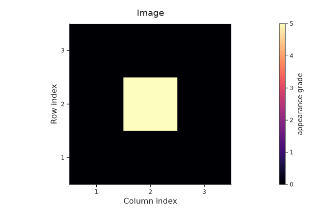
The horizontal axis is the matrix's column index; the vertical axis is its row index, increasing upward. Each coloured tile represents one closed square. Its edges and vertices are included when it appears. The outside boundary is not identified with the opposite side: this is a nonperiodic array.
Watch the hole appear and fill
At parameter $t$, include every square whose grade is at most $t$, together with its edges and vertices. This growing family is a sublevel filtration. In symbols,
\[K_t = \bigcup_{\mathrm{values}[i,j]\leq t} \text{square}_{i,j}.\]
The expression values .<= t compares every array entry with t. Int.(...) converts its true/false entries to a numeric image. Below, 0 means an absent square and 1 means a present square. Every snapshot uses the same coordinates and the same colour range. These are masks of this particular top-cell cubical construction, not a general filtered-complex viewer.
Begin at $t=-1$. The fixed colorrange=(0, 1) lets the same colours mean absent and present in every snapshot, including the entirely empty and entirely full images.
before = values .<= -1
@assert count(before) == 0
before_image = OP.ImageNd(Int.(before))
OP.visualize(before_image; colorrange=(0, 1),
    colorbar_label="present (1) / absent (0)")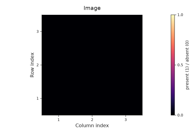
At −1, no square has appeared. Before running the next cell, predict what is present at 0.
ring = values .<= 0
@assert count(ring) == 8 && !ring[2, 2]
ring_image = OP.ImageNd(Int.(ring))
OP.visualize(ring_image; colorrange=(0, 1),
    colorbar_label="present (1) / absent (0)")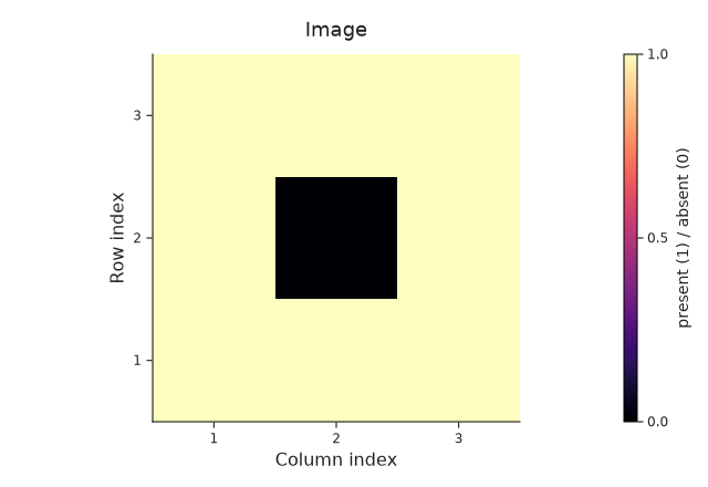
The boundary squares form one connected ring surrounding a hole. It stays this way for every parameter from 0 up to, but not including, 5.
filled = values .<= 5
@assert count(filled) == 9
filled_image = OP.ImageNd(Int.(filled))
OP.visualize(filled_image; colorrange=(0, 1),
    colorbar_label="present (1) / absent (0)")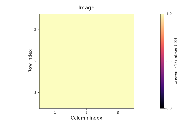
At 5 the center is already present, so the hole has disappeared. The squares and their boundary curves have not vanished; what changed is that a loop around the hole can now be filled by squares.
Compute and read the answer
Homology turns these geometric questions into vector spaces. In degree zero, it records connected components. In degree one, it records loops modulo loops that bound filled regions. A vector in one of these spaces is a homology class. Here the ring has one independent degree-one class, which disappears when the center fills.
cubical_persistence follows these classes through the filtration. We explicitly choose square (top-cell) input, sublevels and nonperiodic boundaries. This ordinary-persistence computation uses the two-element coefficient field $\mathbb{F}_2$: coefficients are 0 or 1 and addition is modulo 2. It returns a PersistenceDiagram, which stores intervals; this direct route does not construct an EncodingResult.
diagram = OP.cubical_persistence(values;
    input=:top_cells, order=:sublevel, periodic=false)
holes = OP.finite_intervals(diagram; dim=1)
@assert holes == [(0, 5)]
@assert isempty(OP.essential_births(diagram; dim=1))
holes
1-element Vector{Tuple{Int64, Int64}}:
(0, 5)The pair (0, 5) means the interval $[0,5)$: the class is present at its birth, 0, and absent at its death, 5. dim=1 selects homological degree one. This agrees with the three snapshots.
A barcode draws that interval on the parameter axis. kind=:barcode selects this view of the computed result; dim=1 selects the holes. The figure chooses its own limits around the interval. A filled circle includes the birth; an open circle excludes the death.
OP.visualize(diagram; kind=:barcode, dim=1)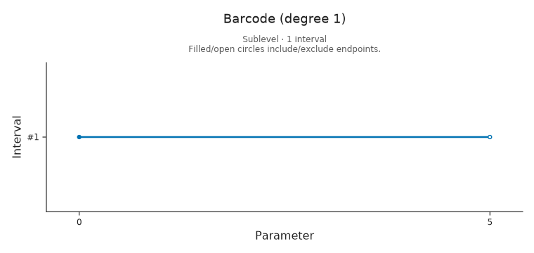
A persistence diagram records the same interval as the point (birth, death) = (0, 5). Its height above the diagonal is read in these parameter coordinates; it is not the geometric size of the hole. A point on the diagonal would have equal birth and death and would not represent a nonzero interval here.
OP.visualize(diagram; kind=:persistence_diagram, dim=1)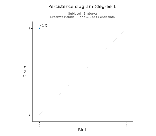
What happened to the connected component? It was born at 0 and never dies in this filtration. Such an interval is called essential. The array stops changing after 5, and the final filled square stays connected at all later parameter values.
components = OP.persistence_intervals(diagram; dim=0)
@assert OP.essential_births(diagram; dim=0) == [0]
@assert isempty(OP.finite_intervals(diagram; dim=0))
components
1-element Vector{Tuple{Int64, Union{Float64, Int64}}}:
(0, Inf)OP.visualize(diagram; kind=:barcode, dim=0)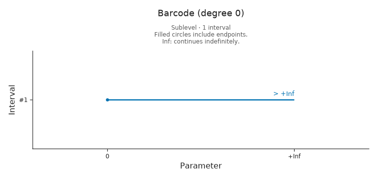
The essential mark means continuation to $+\infty$. The figure has a finite width; its edge does not kill the component. Conversely, the hole really dies at 5. Keeping those two endpoint meanings separate is part of reading a barcode.
Predict a change, then compare
Suppose the central square appears at 3 instead of 5. Before computing, write down the new degree-one interval. Does the essential connected component change?
The next cell checks the prediction. copy keeps the original array available for comparison.
earlier_values = copy(values)
earlier_values[2, 2] = 3
earlier_diagram = OP.cubical_persistence(earlier_values;
    input=:top_cells, order=:sublevel, periodic=false)
@assert values[2, 2] == 5
@assert OP.finite_intervals(earlier_diagram; dim=1) == [(0, 3)]
@assert isempty(OP.essential_births(earlier_diagram; dim=1))
@assert OP.essential_births(earlier_diagram; dim=0) == [0]
@assert isempty(OP.finite_intervals(earlier_diagram; dim=0))
(; original=holes, changed=OP.finite_intervals(earlier_diagram; dim=1))
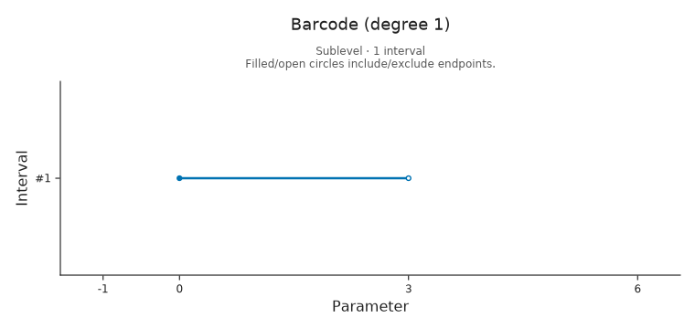
(original = [(0, 5)], changed = [(0, 3)])The hole is born at the same parameter and dies earlier, giving $[0,3)$. The component still begins at 0 and remains essential. Compare the original barcode first, then the changed one. Both use the window −1 to 6; the shorter bar therefore reflects the changed input, not a rescaled axis.
This is where window=(-1, 6) becomes useful: we set it explicitly for both figures. display shows each figure because this cell has two results to show.
display(OP.visualize(diagram; kind=:barcode, dim=1, window=(-1, 6)))
display(OP.visualize(earlier_diagram; kind=:barcode, dim=1, window=(-1, 6)));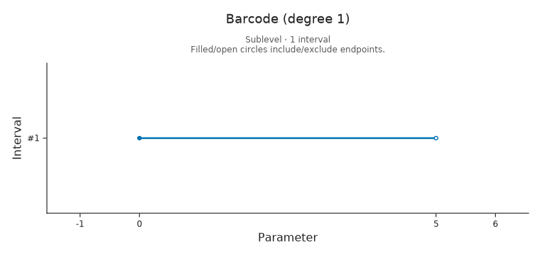
A common mistake: treating the same matrix as vertex values. input=:vertices defines a different filtration. The masks above describe squares and their faces, so our computation deliberately uses input=:top_cells. Similarly, periodic boundaries would change the space.
Optional: Prepare a figure for sharing
The main result is complete. You can skip this section and continue to the second-parameter question below. The earlier figures used the package defaults. For a slide or report, VisualStyle lets us choose larger text, and size sets the canvas width and height in pixels. These choices change the presentation; dim and the comparison window still specify what we are viewing.
We preview the style once before exporting it. This style applies only to calls where we pass it; it does not change later figures globally.
style = OP.VisualStyle(fontsize=18)
OP.visualize(diagram; kind=:barcode, dim=1, window=(-1, 6),
    style=style, size=(760, 360))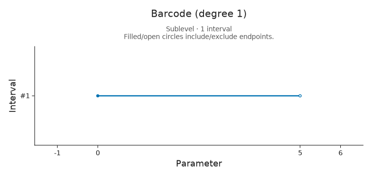
The notebook already retains its displayed figures. To save a separate PNG, use save_visual with the same view, style and size. The files go in tamerop_outputs/ring under your working directory. export_path gives the saved file location.
png = OP.save_visual(joinpath("tamerop_outputs", "ring"), "ring-barcode", diagram;
    kind=:barcode, dim=1, window=(-1, 6),
    style=style, size=(760, 360), format=:png)
@assert isfile(OP.export_path(png))
OP.export_path(png)"tamerop_outputs/ring/ring-barcode.png"SVG keeps the drawing sharp when resized. Change only the file format to keep the same mathematical view and styling.
svg = OP.save_visual(joinpath("tamerop_outputs", "ring"), "ring-barcode", diagram;
    kind=:barcode, dim=1, window=(-1, 6),
    style=style, size=(760, 360), format=:svg)
@assert isfile(OP.export_path(svg))
OP.export_path(svg)"tamerop_outputs/ring/ring-barcode.svg"What changes with a second parameter?
We have followed one growing shape, recognized a birth and a death, and checked that its interval changes as predicted. These bars describe this one-parameter persistence module; they do not identify unique geometric cycle representatives.
With two independently varying parameters, one coordinate can increase while another decreases. Some parameter pairs become incomparable, so one timeline no longer suffices. We must keep the vector spaces and the maps between comparable parameters. A finite encoding is a way to retain that information in a finite description.
Continue with why two parameters change the problem to see how independent thresholds replace a single timeline with a partial order. For the input and endpoint conventions of the computation just completed, consult the ordinary-persistence guide.