Finite encodings: recovering a module from finite data
A persistence module retains a vector space at each parameter and a compatible linear map for each comparison. Over the real plane, there are infinitely many parameters. How can we keep the whole module in a form that a computer can use?
A finite encoding answers this question by assigning parameters to finitely many labels. The labels form a poset, and a module on that poset supplies the spaces and maps. The assignment tells us how to recover them at the original parameters. It is an essential part of the description.
We will build two encodings of the same square-supported module and check what they recover. You need the notions of a poset, a structure map, and composition, together with basic linear algebra. The short bridge why two parameters change the problem introduces these ideas; persistence modules develops the definitions in detail. Either route leads here. No Julia installation is needed; the final sections connect the mathematics to TamerOp's result objects.
Specify the module before encoding it
Let $Q=\mathbb{R}^2$ with coordinatewise order. Fix the coefficient field $\mathbb{k}=\mathbb{Q}$ and the closed square $S=[0,2]^2$. Our module has one independent vector at each parameter in $S$, and no nonzero vectors elsewhere:
\[M(q)= \begin{cases} \mathbb{k}, & q\in S,\\ 0, & q\notin S. \end{cases}\]
The coefficient field has changed from F₂ in the ring example to ℚ here. The parameters still range over all real pairs; coefficients inside a vector space are a separate choice from the coordinates indexing that space. We are specifying this module directly, without claiming that the earlier ring calculation produced it.
We must also specify the maps. For $q\leq r$, let $M(q\leq r)$ be the identity on $\mathbb{k}$ when both points lie in $S$. Otherwise it is the unique zero map between the stated source and target spaces. The matrix of a map has one row per target basis vector and one column per source basis vector:
| Source and target | Structure map | Matrix size |
|---|---|---|
| Both inside $S$ | Identity | $1\times1$ |
| Outside to inside | Zero map $0\to\mathbb{k}$ | $1\times0$ |
| Inside to outside | Zero map $\mathbb{k}\to0$ | $0\times1$ |
| Both outside | Unique map $0\to0$ | $0\times0$ |
Each row assumes that the original parameters are comparable in the stated direction. The unique endomorphism of the zero space is both its zero map and its identity map.
These rules define a module because they respect composition. If $q\leq r\leq s$ and both endpoints lie in the square, the intermediate point lies there too: each of its coordinates is between the corresponding endpoint coordinates. The three maps are identities. In every other case at least one endpoint space is zero, so both the direct map and the composite are zero. A subset with this between-points property is called order-convex.
The square is the module's support, meaning the set where its stalks are nonzero. It is not a restriction on the query domain. Points outside the square still have well-defined zero spaces. The boundary also matters: $(0,0)$, $(2,2)$, and every point along the four edges belong to the support. This is a closed square, distinct from the half-open interval $[0,5)$ in the ring example.
A finite model with nine labels
For each real coordinate $x$, record which of three bands contains it:
\[b(x)= \begin{cases} L, & x<0,\\ C, & 0\leq x\leq2,\\ H, & x>2. \end{cases}\]
The letters mean lower, central, and higher, with order $L<C<H$. Increasing $x$ can keep its label unchanged or move it upward in this order; it cannot move it downward.
Take the nine pairs of band labels as a finite poset $P_9=\{L<C<H\}\times\{L<C<H\}$, ordered coordinatewise. Assign a parameter $q=(x,y)$ its label by
\[\pi_9(x,y)=(b(x),b(y)).\]
If $q\leq r$, then $\pi_9(q)\leq\pi_9(r)$: both coordinate labels move in the permitted direction. A map with this property is order preserving. A fiber of $\pi_9$ is the set of parameters assigned to one label; here the fibers are exactly the nine regions specified by the band pairs.
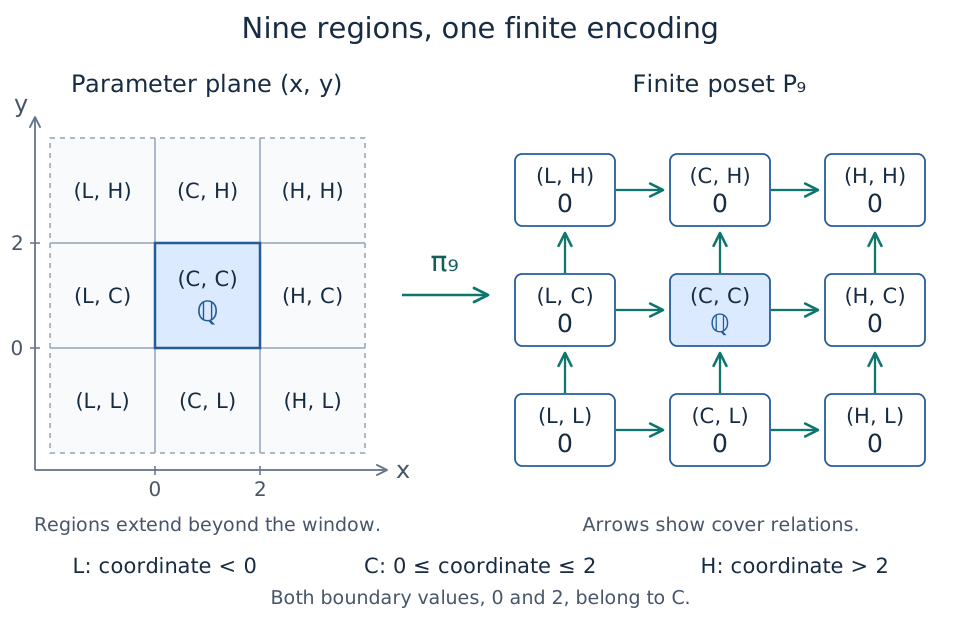
The left panel shows part of the original plane; its outer regions extend beyond the displayed window. Coordinates equal to 0 or 2 belong to band C. The right panel is the finite poset of labels, with spaces attached. Arrows show its immediate comparisons, called covers; longer comparisons follow by composition. This is an authored schematic, not a claim about the number or numbering of labels returned by the package.
Define a module $N_9$ on this finite poset by placing $\mathbb{k}$ at $(C,C)$ and zero at the other eight labels. Every map between distinct comparable labels is zero, since at least one of its spaces is zero. Every label also has its identity map, including the identity of $\mathbb{k}$ at $(C,C)$.
We can now recover a space at any original parameter by first finding its label, then using the space stored there:
| Parameter $q$ | Label $\pi_9(q)$ | Recovered space $N_9(\pi_9(q))$ |
|---|---|---|
| $(-1,1)$ | $(L,C)$ | $0$ |
| $(1/4,1/2)$ | $(C,C)$ | $\mathbb{k}$ |
| $(1,3/2)$ | $(C,C)$ | $\mathbb{k}$ |
| $(2,2)$ | $(C,C)$ | $\mathbb{k}$ |
| $(3,1)$ | $(H,C)$ | $0$ |
The same procedure recovers maps. The points $(1/4,1/2)\leq(1,3/2)$ have the same central label, so their map is the identity at $(C,C)$. For $(1,3/2)\leq(3,3/2)$, use the finite map from $(C,C)$ to $(H,C)$: the zero map from $\mathbb{k}$ to zero. For $(-1,1)\leq(0,1)$, use the map from $(L,C)$ to $(C,C)$, whose matrix has one row and no columns.
An infinite collection of space and map queries is now answered by a finite module together with an explicit rule for finding labels. The rule works throughout ℝ²; this construction is not limited to the sample points in the table.
What the definition requires
For a module $M$ on a poset $Q$, a finite encoding consists of a finite poset $P$, a module $N$ on $P$ with finite-dimensional stalks, and an order-preserving map $\pi:Q\to P$, such that
\[M\cong\pi^*N=N\circ\pi.\]
This is the finite-encoding definition in Ezra Miller's Homological algebra of modules over posets, Definition 4.1. The map $\pi$ is often called the encoding map or classifier: it assigns an original parameter to a finite label.
The notation $\pi^*N$, called the pullback of $N$, means the module on $Q$ obtained by those lookups:
\[(\pi^*N)(q)=N(\pi(q)),\qquad (\pi^*N)(q\leq r)=N(\pi(q)\leq\pi(r)).\]
Order preservation ensures that the finite comparison on the right exists whenever the original comparison on the left exists. The identity and composition rules for $N$ then give the corresponding rules for the pullback. For example, a chain $q\leq r\leq s$ is sent to a chain of labels, so the finite model's composite agrees with its direct map.
The symbol $\cong$ allows the recovered spaces to use different bases from the original ones. More precisely, there must be invertible linear maps $\alpha_q:M(q)\to N(\pi(q))$ such that, for every $q\leq r$,
\[\alpha_r\circ M(q\leq r) =N(\pi(q)\leq\pi(r))\circ\alpha_q.\]
Starting with a vector in $M(q)$, we can either follow the original map and then change coordinates, or change coordinates first and follow the finite map. Both routes must give the same vector. This compatibility is called naturality. It is stronger than merely finding vector spaces of the same dimensions. In the original bases, the recovered map is
\[M(q\leq r) =\alpha_r^{-1}\circ N(\pi(q)\leq\pi(r))\circ\alpha_q.\]
For our square, we used the same copy of $\mathbb{k}$ and the same basis throughout the support, so the identifications can be taken to be identities. In a computation, different basis choices can change matrix entries while these compatibility equations still hold.
Keeping $P$ and $N$ without $\pi$ would leave us unable to locate an original parameter. Keeping $P$ and $\pi$ without the maps of $N$ would leave us unable to follow vectors. The finite poset, its module, and the encoding map all contribute to the representation.
The definition makes the poset and its vector-space data finite. Computation also needs a usable description of $\pi$, such as the inequality tests in our example. The existence of an abstract encoding alone does not supply an algorithm for evaluating its classifier.
Why equal dimensions do not define the labels
The square has only two stalk dimensions, zero and one. Could we therefore use just an exterior label $z$ and an interior label $a$?
Consider the comparable chain
\[(-1,1)\leq(1,1)\leq(3,1).\]
Its proposed labels would be $z,a,z$. Order preservation would force both $z\leq a$ and $a\leq z$. Antisymmetry in a poset would then force $z=a$. But one label cannot carry both a zero-dimensional and a one-dimensional space. This two-label assignment cannot be an encoding.
Thus even zero spaces may need several labels to record how they lie before, after, or beside the nonzero part. More generally, a partition by dimensions need not respect either the parameter order or the structure maps. A picture colored only by dimension does not provide an encoding map automatically.
Conversely, equal labels do not force original parameters to be comparable. The points $(1/4,3/2)$ and $(3/2,1/4)$ both have label $(C,C)$, but neither precedes the other. The identity at that finite label supplies a map only when we start with a valid comparison in $Q$. Order preservation is a one-way implication; it does not reconstruct the order of the original parameters from their labels.
Another valid encoding has four labels
The nine-label model is convenient to draw, but a finite encoding is not unique. For this same square, record two yes-or-no facts about $q=(x,y)$:
\[u(q)= \begin{cases}1,&x\geq0\text{ and }y\geq0,\\0,&\text{otherwise},\end{cases} \qquad c(q)= \begin{cases}1,&x>2\text{ or }y>2,\\0,&\text{otherwise}.\end{cases}\]
The first bit says that both lower thresholds have been reached. The second says that at least one upper threshold has been exceeded. Both bits can change from 0 to 1 as parameters increase, but cannot change back. Notice the strict inequality in $c$: coordinates equal to 2 remain inside the closed support.
Set $\pi_4(q)=(u(q),c(q))$ and order the four possible pairs coordinatewise, using $0<1$. All four pairs occur, so they form the four-label poset $P_4$. The map $\pi_4:Q\to P_4$ is order preserving. Put $\mathbb{k}$ at the label $(1,0)$ and zero at the other three labels to obtain a finite module $N_4$; as before, maps between distinct comparable labels are zero and endomorphisms are identities.
| Signature $(u,c)$ | Example parameter | Space |
|---|---|---|
| $(0,0)$ | $(-1,1)$ | $0$ |
| $(1,0)$ | $(1,1)$ | $\mathbb{k}$ |
| $(0,1)$ | $(-1,3)$ | $0$ |
| $(1,1)$ | $(3,1)$ | $0$ |
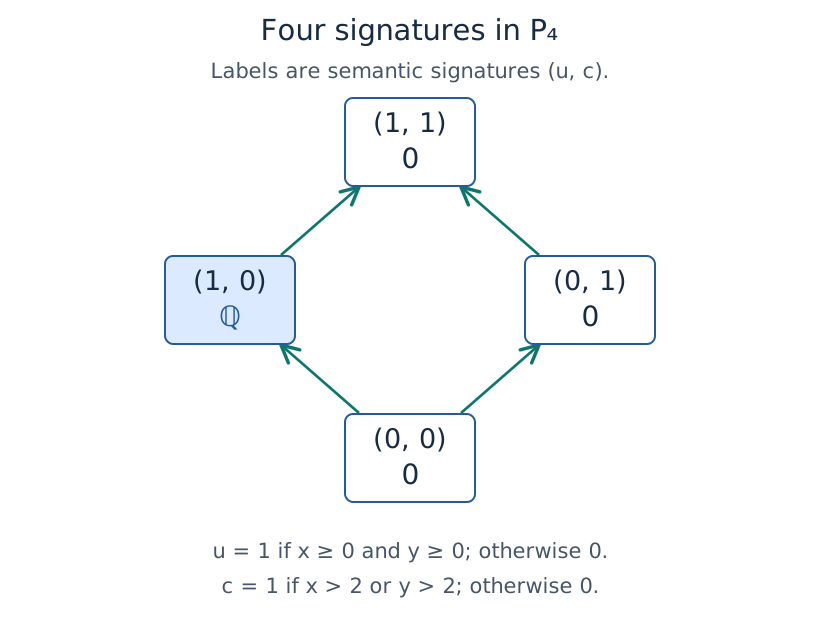
This authored schematic uses the two mathematical bits as labels, not numeric vertex IDs from a package result. Arrows show the finite order. Every drawn arrow has a zero structure map, while the identity at the nonzero label recovers maps between comparable points inside the square. Both routes around the diamond compose to the unique map between its zero endpoint spaces.
The condition $u=1,c=0$ is exactly $0\leq x\leq2$ and $0\leq y\leq2$. Thus stalk lookup recovers $M$ everywhere. For comparable points inside the square it recovers an identity; in every other case it recovers the required zero map. This proves that the four-label construction encodes the same module as the nine-label construction.
A label need not describe one connected geometric region. The signature $(0,1)$ covers both the upper-left region $x<0,y>2$ and the lower-right region $x>2,y<0$. These disconnected pieces can share a label in this encoding. There is no requirement that the regions be rectangular cells or that the finite diagram reproduce their Euclidean positions.
Relate the two finite models
There is an explicit map $\rho:P_9\to P_4$ connecting the models. Given a band pair, set $u=1$ when neither coordinate label is $L$, and set $c=1$ when at least one is $H$:
| Nine-label regions | Four-label signature |
|---|---|
| $(L,L)$, $(L,C)$, $(C,L)$ | $(0,0)$ |
| $(C,C)$ | $(1,0)$ |
| $(L,H)$, $(H,L)$ | $(0,1)$ |
| $(C,H)$, $(H,C)$, $(H,H)$ | $(1,1)$ |
Moving upward in $P_9$ cannot turn either bit from 1 back to 0, so $\rho$ is order preserving. The label assignments satisfy
\[\pi_4=\rho\circ\pi_9.\]
We can therefore label a point directly by its two bits, or first find its band pair and then apply $\rho$. Both routes give the same label. The spaces and maps also agree:
\[N_9=\rho^*N_4,\qquad M=\pi_9^*N_9=\pi_4^*N_4\]
with the explicit choices made here. For example, several zero labels can merge under $\rho$ because their finite maps then become the identity on the zero space, which is also its unique zero map. Checking the labels and the maps establishes the comparison; counting nine versus four vertices would not establish it.
Figure placeholder: compare the two encodings. A linked view will color the nine regions by their four signatures. Selecting a point or a comparable pair will trace both routes through $\pi_9$, $\rho$, and $\pi_4$, displaying the same recovered spaces and maps. The separated pieces with signature $(0,1)$ will share a color and an explicit label.
What the package returns for this example
The inspection notebook constructs the square using a region defined by lower bounds, a region defined by upper bounds, and a one-by-one coefficient matrix $[1]$ over ℚ. With backend=:pl_backend and poset_kind=:signature, the encoder returns a poset with the four signatures just described, ordered as the diamond. The second bit records the complement of membership in the region defined by the upper bounds. Taking the complement makes that bit increase with the parameters. The indicator-presentations chapter explains this input construction.
The returned numeric vertex IDs are bookkeeping choices. Find labels with the returned encoding map and inspect the actual poset. Neither the nine-region schematic nor a particular ordering of the four signatures is a requirement on all encoders. A different representation can still satisfy the same recovery equations.
The notebook follows boundary, interior, and exterior points into the returned model, then recovers maps for comparable pairs. It also distinguishes an incomparable pair that shares a label. The arguments above explain why the models recover the module throughout ℝ², beyond those selected queries. The geometric endpoints and query coordinates in this example are exactly representable as Float64, while the linear algebra uses ℚ. Arbitrary real geometric inputs need not be represented exactly by floating-point coordinates; see exact grades for the supported contracts.
What recovery guarantees
Once the represented module $M$ is fixed, a finite encoding recovers its stalks and its structure maps up to the compatible identifications described above. In particular, it recovers the dimensions of stalks and the ranks of maps at specified comparable parameters. The finite labels themselves are not persistent classes, and an encoding is not an interval decomposition: one label can carry a higher-dimensional space and nontrivial matrices can connect different labels in other examples.
Earlier modeling choices still matter. Selecting a filtration, truncating a complex, or changing the grid used to define an input can change $M$. An encoding of the chosen module does not by itself undo those changes. Likewise, replacing the square's upper closed boundary by an open one would change its stalk at $(2,2)$; it would describe a different module, not merely rename this encoding's labels.
Recovering a module also does not identify all algebraic computations over different base posets. In particular, Ext or Tor over a finite encoding poset need not equal the corresponding groups over the original parameter poset, or over another encoding. These computations require their own category and comparison hypotheses; the category guide develops that distinction.
Why the name TamerOp?
TamerOp stands for Toolkit for Algebraic Module Encodings over $\mathbb{R}^n$ and Other Posets. It implements constructions from Ezra Miller's theory of modules over posets. Finite encodings are the central objects connecting its constructions, algebra, and summaries.
The name also recalls tameness, a finiteness condition on how a module varies, including its maps. For modules with finite-dimensional stalks, Ezra Miller's finite-encoding theorem relates finite encodings to finite constant subdivisions: partitions into finitely many regions whose spaces can be identified while keeping the maps between regions consistent. Encoding fibers form such a subdivision, with the additional organization supplied by an order-preserving map. A given constant subdivision need not itself provide these fibers. Grouping all exterior zero spaces above illustrates why order compatibility is an additional requirement on the labels. The tameness and scope chapter develops the hypotheses and the connections to presentations and resolutions. The theorem's generality does not imply an implemented encoder for every abstract input.
For the square, the construction already supplies the required finiteness. Filtrations of a fixed finite complex also supply it automatically. The follow-on explanation why finite computations stay tame shows why, and how encoding the relevant maps lets kernels, images, and homology remain finite. You can read it directly from this chapter or after the full tameness development.
From an input to the encoded object
The mathematical description helps us recognize what a package result must contain. Inputs can come from a point cloud, graph, or image with a chosen filtration, or from a presentation specifying a module through algebraic pieces and maps. An already finite-poset module is another starting point. For supported inputs, the public workflow encode produces an EncodingResult connecting the finite object to its parameter domain and recorded construction.
| Mathematical question | Operation |
|---|---|
| What does this result contain? | describe(enc) |
| Which conventions and construction were recorded? | provenance(enc) |
| What is the finite poset $P$? | encoding_poset(enc) |
| What is the assignment $\pi$ from original parameters? | encoding_map(enc) |
| What are the dimensions at finite labels? | dimensions(enc) |
| What is the finite module $N$, including its maps? | encoding_module(enc) |
Some ingestion results defer expensive calculations: dimensions computes the dimensions, while encoding_module explicitly computes the module and its maps if needed. The inspection guide explains this distinction. A request for an intermediate stage, or a direct ordinary-persistence calculation, should not be mistaken for a completed EncodingResult.
Recover the square in a computation
We have built two finite models by hand and identified the data a package result must retain. Continue with inspect spaces and maps to follow an original parameter into the returned finite poset, recover its space, and inspect the map for a comparable pair. The square gives known answers against which to interpret each query and figure.
To understand the input construction first, read indicator presentations. It explains how the square's lower and upper regions, linked by the coefficient $1$, specify the module, then combines two overlapping squares to produce inclusion and projection maps.