Indicator presentations: building a module from regions and a matrix
The finite-encodings chapter began with a module supported on a square and explained how finite data recover its spaces and maps. To give that module to an encoder, we need a finite description of the input itself. How can regions and a small matrix specify a module over the whole real plane?
We will construct the square from two simpler modules, then combine two overlapping squares. The second example has spaces of dimensions one, two, and one along an increasing path. Its maps will explain why the vector visible at the start does not survive to the end, even though neither of the two successive maps is zero.
You need the previous chapters' notions of a poset, a module, and compatible structure maps, together with matrix multiplication. We continue with $Q=\mathbb{R}^2$, coordinatewise order, and coefficient field $\mathbb{k}=\mathbb{Q}$. Parameters are real pairs; matrix entries are rational numbers. No Julia installation is needed to follow the chapter.
Separate the square's lower and upper bounds
Our square is $S=[0,2]^2$. Its inequalities fall into two groups:
\[U=\{(x,y):x\geq0,\ y\geq0\},\qquad D=\{(x,y):x\leq2,\ y\leq2\}.\]
Their intersection is $S$. Each region has a useful relationship to the order. Once a point belongs to $U$, increasing either coordinate keeps it in $U$. A subset with this property is an upset: $q\in U$ and $q\leq r$ imply $r\in U$. For $D$, decreasing coordinates preserves membership. Such a subset is a downset: $r\in D$ and $q\leq r$ imply $q\in D$.
The names describe the direction in which membership persists. In this picture, the lower bounds define the upset, extending toward the upper right; the upper bounds define the downset, extending toward the lower left. Neither region is bounded.
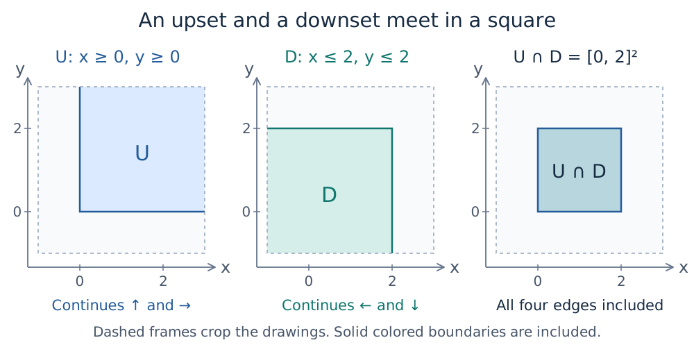
The panels show cropped portions of unbounded regions. The solid boundary lines belong to the regions. Their intersection includes all four edges and corners of the square.
General upsets and downsets need not have a single corner or rectangular boundaries. These particular regions let us introduce the construction without additional geometry.
Turn a region into an indicator module
The indicator module $\mathbb{k}[U]$ puts one copy of $\mathbb{k}$ at each point of $U$ and the zero vector space elsewhere:
\[\mathbb{k}[U](q)= \begin{cases} \mathbb{k},&q\in U,\\ 0,&q\notin U. \end{cases}\]
For a comparison $q\leq r$, its map is the identity if both points lie in $U$, and the unique zero map otherwise. Define $\mathbb{k}[D]$ by the same rule with $D$ in place of $U$.
These are modules, including their maps. Along an increasing sequence of parameters, the upset indicator can change from $0$ to $\mathbb{k}$ but cannot leave its support once it enters. The downset indicator can change from $\mathbb{k}$ to $0$ but cannot reenter after leaving. Consequently, the identity and zero maps compose as required. More generally, an intersection of an upset and a downset is order-convex, the property used to check the square module in the previous chapter.
The bracket notation means a module, rather than just the numerical function recording membership. It includes structure maps. The coefficient $1$ below is also different from a membership bit: it specifies a linear map over $\mathbb{k}$.
Recover the square as an image
Define a map of modules
\[\varphi:\mathbb{k}[U]\longrightarrow\mathbb{k}[D]\]
by multiplication by $1$ wherever both spaces are nonzero. Elsewhere, $\varphi_q$ is the unique zero map between the two spaces. At each parameter:
| Location of $q$ | Source | Target | Matrix of $\varphi_q$ | Image |
|---|---|---|---|---|
| $U\cap D$ | $\mathbb{k}$ | $\mathbb{k}$ | $[1]$ | $\mathbb{k}$ |
| $U\setminus D$ | $\mathbb{k}$ | $0$ | $0\times1$ zero matrix | $0$ |
| $D\setminus U$ | $0$ | $\mathbb{k}$ | $1\times0$ zero matrix | $0$ |
| Outside both | $0$ | $0$ | $0\times0$ matrix | $0$ |
Here the image of a linear map is the subspace of its target consisting of all output vectors. Thus $\operatorname{im}\varphi_q$ has exactly the space we want at $q$.
The pointwise maps $\varphi_q$ must also respect the structure maps. For every $q\leq r$ we require
\[\mathbb{k}[D](q\leq r)\,\varphi_q = \varphi_r\,\mathbb{k}[U](q\leq r).\]
In words, applying $\varphi$ and then moving forward gives the same answer as moving forward and then applying $\varphi$. If $q\in U$ and $r\in D$, upward closure of $U$ and downward closure of $D$ put both points in $U\cap D$; both sides are the identity. Otherwise the source at $q$ or the target at $r$ is zero, so both sides are zero.
This compatibility lets the target structure maps carry images to images. Define $M(q)=\operatorname{im}\varphi_q$, and obtain $M(q\leq r)$ by restricting the target map to that image, with codomain $\operatorname{im}\varphi_r$. We recover the earlier square module: identity maps between comparable points in $S$, and correctly shaped zero maps otherwise.
The compact input is therefore one upset, one downset, and the one-by-one matrix $[1]$. The module is the image of the map they describe. Changing $[1]$ to $[0]$ gives the zero module on the entire plane; the regions alone do not determine the answer.
Several indicators and one coefficient matrix
Now choose a finite list of upsets $U_1,\ldots,U_m$ and downsets $D_1,\ldots,D_n$. Form
\[F=\bigoplus_{i=1}^{m}\mathbb{k}[U_i], \qquad E=\bigoplus_{j=1}^{n}\mathbb{k}[D_j].\]
A direct sum keeps the summands as independent coordinates. At a point belonging to two upsets, for example, $F(q)$ has two independent basis vectors, even if the regions overlap geometrically.
An $n\times m$ matrix $A=(a_{ji})$ specifies a map $\varphi:F\to E$: the block from $\mathbb{k}[U_i]$ to $\mathbb{k}[D_j]$ multiplies by $a_{ji}$ throughout $U_i\cap D_j$. Outside that intersection its pointwise map is zero. We use target downsets as rows and source upsets as columns, so matrices act on column vectors. If an intersection is empty, its block is zero; take the corresponding coefficient to be zero as well.
The same compatibility argument as for the square works for every block. We can therefore define $M=\operatorname{im}\varphi$. A module isomorphic to this image is also said to have the specified presentation.
This particular kind of indicator presentation is called a fringe presentation. In Ezra Miller's terminology, its component maps are connected: each uses one scalar throughout its intersection. For an arbitrary poset, a general map between two indicators can have different scalars on components that cannot be joined by a zigzag of comparisons within the intersection. The single-scalar requirement is part of this presentation convention. See Definitions 3.14–3.17 in Homological algebra of modules over posets.
If you know presentations by generators and relations, keep the output operation in view: here $M$ is an image. A usual presentation $F_1\to F_0\to M\to0$ describes $M$ as a cokernel. These are different ways to specify a module. The terms “birth upsets” and “death downsets” describe the two sides of the fringe construction; they do not assert that its rows and columns are a minimal list of topological events.
Read a stalk from the active rows and columns
At a parameter $q$, let
\[I(q)=\{i:q\in U_i\},\qquad J(q)=\{j:q\in D_j\}.\]
These index the active source and target coordinates. Keep their original list order when forming matrices. Then
\[F(q)=\mathbb{k}^{I(q)},\quad E(q)=\mathbb{k}^{J(q)},\quad \varphi_q=A[J(q),I(q)].\]
The last expression means: retain exactly the rows indexed by $J(q)$ and columns indexed by $I(q)$. Hence
\[M(q)=\operatorname{im} A[J(q),I(q)], \qquad \dim M(q)=\operatorname{rank} A[J(q),I(q)].\]
Rank counts independent output vectors. It can be smaller than either the number of active rows or the number of active columns. Empty row or column sets give zero-dimensional images, with the usual empty matrix shapes.
Recover maps by following target coordinates
When $q\leq r$, upset coordinates can appear and downset coordinates can disappear:
\[I(q)\subseteq I(r),\qquad J(r)\subseteq J(q).\]
The source map inserts zeros in newly available coordinates. The target map projects onto the coordinates that remain in $J(r)$. Restrict this projection to $M(q)$ to obtain $M(q\leq r)$. Its values land in $M(r)$ because the presentation map commutes with the source and target maps.
An image subspace is often stored using its own basis. If $B_q$ and $B_r$ have columns forming bases for the two images in target coordinates, and $P_{q,r}$ is the target projection, the structure matrix $C_{q,r}$ satisfies
\[B_r C_{q,r}=P_{q,r} B_q.\]
This equation says to project each source basis vector and express the answer in the target image basis. The dimensions alone cannot supply $C_{q,r}$. Different basis choices can change its entries while preserving the represented linear map.
Two overlapping squares
Take two pairs of regions:
\[\begin{aligned} U_1&=\{x\geq0,\ y\geq0\},&D_1&=\{x\leq2,\ y\leq2\},\\ U_2&=\{x\geq1,\ y\geq1\},&D_2&=\{x\leq3,\ y\leq3\}, \end{aligned} \qquad A=\begin{bmatrix}1&0\\0&1\end{bmatrix}.\]
Each source coordinate maps only to the matching target coordinate. Consequently,
\[M\cong\mathbb{k}[S_1]\oplus\mathbb{k}[S_2], \qquad S_1=[0,2]^2,\quad S_2=[1,3]^2.\]
Here $\mathbb{k}[S_i]$ uses the identity and zero maps already defined for a square. The dimension is two on the closed overlap $[1,2]^2$, one where exactly one square is present, and zero outside their union.
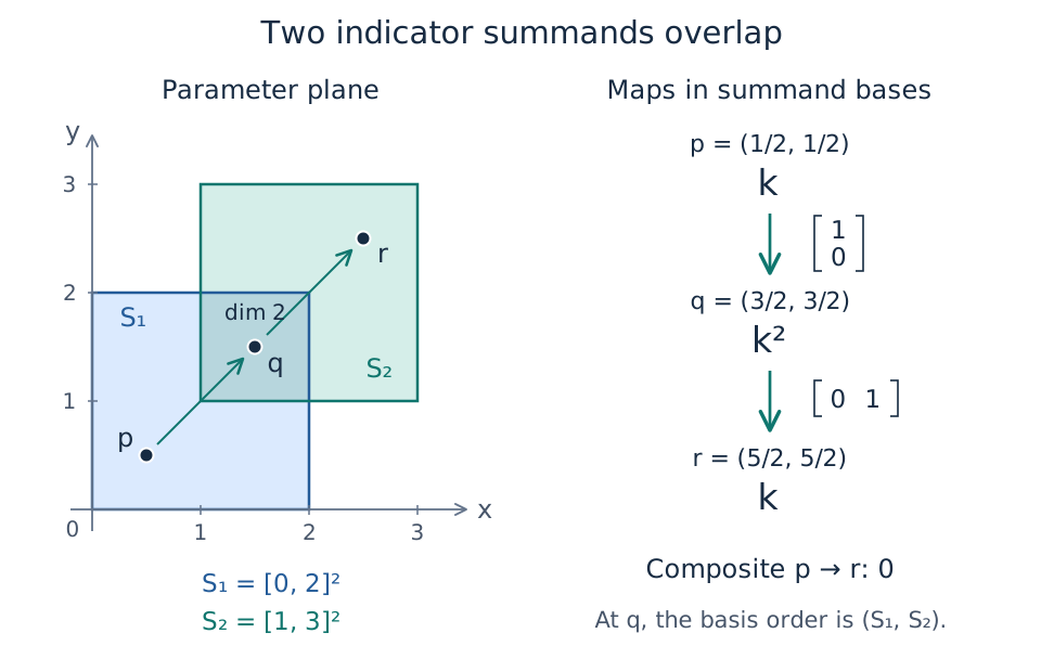
This schematic shows the two summands in different colors. The map diagram uses the summand bases: first-square coordinate first, second-square coordinate second. The zero composite follows from which coordinate survives.
Follow the comparable points $p=(\tfrac12,\tfrac12)\leq q=(\tfrac32,\tfrac32)\leq r=(\tfrac52,\tfrac52)$. The presentation matrices and their images are:
| Parameter | Active upsets $I$ | Active downsets $J$ | Presentation matrix | Image in target coordinates |
|---|---|---|---|---|
| $p$ | $\{1\}$ | $\{1,2\}$ | $\begin{bmatrix}1\\0\end{bmatrix}$ | $\operatorname{span}(e_1)\subseteq\mathbb{k}^2$ |
| $q$ | $\{1,2\}$ | $\{1,2\}$ | $\begin{bmatrix}1&0\\0&1\end{bmatrix}$ | $\mathbb{k}^2$ |
| $r$ | $\{1,2\}$ | $\{2\}$ | $\begin{bmatrix}0&1\end{bmatrix}$ | $\mathbb{k}$, in the $D_2$ coordinate |
The target has two coordinates at $p$, but the image has dimension one. At $r$ the source still has two coordinates, but the image again has dimension one. This is why we take ranks of the selected matrices.
In the stated summand bases the module maps are
\[\mathbb{k} \xrightarrow{\left[\begin{smallmatrix}1\\0\end{smallmatrix}\right]} \mathbb{k}^2 \xrightarrow{\left[\begin{smallmatrix}0&1\end{smallmatrix}\right]} \mathbb{k}.\]
The first map preserves the first-square vector in the overlap. The second retains only the second-square vector after the first square has ended. Thus both maps have rank one, but
\[M(p\leq r)=M(q\leq r)\,M(p\leq q) =\begin{bmatrix}0&1\end{bmatrix} \begin{bmatrix}1\\0\end{bmatrix} =\begin{bmatrix}0\end{bmatrix}.\]
The last matrix is a $1\times1$ zero map between nonzero spaces. It differs from a map whose source or target is zero. The vector at $p$ has disappeared by $r$; the nonzero space at $r$ belongs to the other summand. A dimension plot by itself does not show this.
Check a point away from the diagonal
At $t=(\tfrac12,\tfrac52)$, only $U_1$ and $D_2$ are active. There is one source coordinate and one target coordinate, yet
\[\varphi_t=A[\{2\},\{1\}]=[0],\qquad M(t)=0.\]
Geometrically, $t$ lies in neither square. Algebraically, the off-diagonal coefficient is zero. Merely checking whether some upset and some downset are present would give the wrong answer.
Boundaries provide another useful check. Both $(1,1)$ and $(2,2)$ lie in both closed squares, so both stalks have dimension two. The query domain remains all of $\mathbb{R}^2$, including parameters outside the support.
Inspect the calculation in the package
The inspection notebook constructs these two square summands and follows the hand calculation with the reusable :presentation_inspector recipe. A static selection shows membership in a chosen upset and downset on the actual encoding regions, identifies active rows and columns of the full coefficient matrix, and displays their block. Requesting an image basis adds its embedding in the active target coordinates. At $t$, that basis has shape $1\times0$: the ambient target has one coordinate, and its image has no basis vectors. The active $1\times1$ zero block is shown as zero, rather than as missing support.
For a comparable pair, the figure displays the endpoint blocks and image bases, the coordinate projection, and the induced map. The notebook checks the equation $B_r C_{q,r}=P_{q,r}B_q$ and multiplies the two successive induced maps to obtain the zero composite. The projection and the induced map can have different shapes: their source and target coordinates describe different spaces, even when both arise from the same presentation.
The package exposes these ingredients through presentation_stalk, active_rows, active_columns, presentation_matrix, and image_basis. presentation_map with source and target returns the endpoint stalks, ambient_projection, and induced_map. A stalk query computes only the active block and its rank unless basis=true; a map query computes the bases it needs. See the spaces-and-maps guide for calling conventions and supported inputs.
These queries inspect the finite presentation retained by the encoding, in its chosen image bases. Those bases need not be the coordinates of an arbitrary stored module, and they do not identify input cycles. Inspection does not invent a presentation when none is retained. It also works from finite labels without a geometric parameter picture.
The notebook also connects these panels through a live inspection session. Selecting a point or pair updates the finite-poset, support, and matrix views; changing between module and presentation views preserves the query. Exact coordinate entry resolves boundaries that a pointer cannot distinguish. These controls require WGLMakie and a running Julia process; the selected state can be saved as a static figure.
Figure placeholder: follow a chosen vector. A three-point view will follow a vector from the first square into the overlap and then into the second square. It will place each vector beside the matrix acting on it, showing how two nonzero maps can have zero composite.
How the presentation leads to a finite encoding
A finite list of regions supplies finitely many membership patterns. For the square, the previous chapter used the two increasing bits
\[u(q)=\mathbf{1}_{U}(q),\qquad c(q)=\mathbf{1}_{Q\setminus D}(q).\]
Membership in an upset is increasing; membership in a downset is decreasing, so its complement gives an increasing bit. For our closed $D$, leaving means $x>2$ or $y>2$, with strict inequalities.
For a general finite fringe presentation, collect one such bit for each upset and each complemented downset. The resulting map into a finite Boolean poset is order-preserving. A pattern determines the active rows and columns, their image space, and the coordinate projections for comparable patterns. These data give a finite module whose pullback recovers the presented module.
This explains the connection between the two descriptions. The presentation supplies regions and coefficients. An encoding supplies a finite poset, a module on it, and a map assigning original parameters to finite labels. The coefficient matrix is needed even after the membership patterns have been found.
The package can organize the finite representation according to the chosen encoder. Use its returned classifier and poset rather than assuming a particular list or numbering of labels. In particular, the square's nine-region illustration remains valid even though the signature encoder used in the notebook returns four labels.
Recognize the construction in TamerOp
For the examples here, the public workflow takes the region lists, the coefficient matrix, and encoding options: OP.encode(upsets, downsets, coefficients, options), where OP denotes TamerOp. The mathematical ingredients correspond to:
| Ingredient | Package expression or choice |
|---|---|
| Upset with lower corner $(0,0)$ | TamerOp.Advanced.BoxUpset([0.0, 0.0]) |
| Downset with upper corner $(2,2)$ | TamerOp.Advanced.BoxDownset([2.0, 2.0]) |
| Rational linear algebra | TamerOp.CoreModules.QQField() and coefficients of type TamerOp.QQ |
| Selected encoder | TamerOp.Advanced.EncodingOptions with backend=:pl_backend, poset_kind=:signature, and the chosen field |
| Finite poset, classifier, and module | encoding_poset(enc), encoding_map(enc), encoding_module(enc) |
| Dimensions at the finite labels | dimensions(enc) |
The region constructors describe unbounded upsets and downsets despite the word Box in their names. Their intersection gives a bounded square. To query an original parameter, locate its finite label with TamerOp.Advanced.locate on the returned classifier. For comparable parameters, obtain N = OP.encoding_module(enc) and inspect its map with TamerOp.Advanced.structure_map(N; source=i, target=j). The matrix is expressed in the returned module's bases; relate those bases to any independently chosen mathematical bases before comparing entries.
The notebook uses integer and half-integer geometric coordinates, represented exactly as Float64. This is separate from the exact rational coefficient field. See exact grades for the package's broader geometric input contracts.
What this construction prepares us to ask
The identity coefficient matrix made our second example a direct sum of two square modules. General matrices couple source and target summands, and general upsets and downsets need not bound rectangles. A fringe presentation does not assert a rectangle decomposition or provide a multiparameter barcode classification.
We can now distinguish three tasks: describe a module by regions and a map, construct a finite encoding of it, and inspect the recovered spaces and maps. The next mathematical question is which modules admit such finite descriptions. The tameness and scope chapter explains the finiteness hypotheses relating presentations, encodings, and resolutions, together with the distinction between existence theorems and implemented constructions.
To work through the construction in Julia first, follow inspect spaces and maps. It connects the active coefficient blocks, their image bases, and the induced maps in the overlapping-square example.