Exact rational coordinates
Many computations with a finite encoded module eventually ask the same linear-algebra question: how do we express these vectors in this basis? An image basis identifies a subspace, but a map into that subspace must also be written in its coordinates. Homology adds another step: express a cycle in a cycle basis, then pass to coordinates modulo boundaries.
This account follows TamerOp's exact rational full-column solver, the reusable data behind it, and its specialization for homology coordinates. The central choice is to use a small invertible row minor to recover candidate coordinates, while retaining a check against the original problem. Its performance depends on where that work happens, which data can be reused, and when conversion to a native exact-arithmetic library pays for itself.
The reusable-factor path is developed first. Backend selection explains when a direct solve takes the modular route instead.
The problem and its certificate
Let $B\in\mathbb Q^{m\times n}$ have independent columns, with $m\geq n$. Its columns are the chosen basis of a subspace of $\mathbb Q^m$. Given $Y\in\mathbb Q^{m\times r}$, we seek
\[B X=Y,\qquad X\in\mathbb Q^{n\times r}.\]
There is at most one answer. There is an answer precisely when every column of $Y$ belongs to the image of $B$. A coordinate routine therefore has two jobs: recover the coefficients and establish that they describe the supplied vectors. This is an exact membership question. A small floating-point residual does not settle it.
TamerOp selects $n$ independent rows of $B$, in an ordered index list $I$. The square matrix $S=B[I,:]$ is invertible, so any solution must satisfy
\[X=S^{-1}Y[I,:].\]
This gives a candidate without eliminating the whole augmented matrix on every query. It does not, by itself, establish membership. If $E_I$ selects the rows in $I$, then $L=S^{-1}E_I$ satisfies $LB=I_n$. Thus $BL$ is a projection onto the image of $B$, and the remaining question is whether $BLY=Y$. In the general solver this becomes the complete check $BX=Y$.
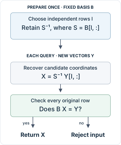
The candidate uses selected rows; the certificate covers the original equation. Reuse is valid only while the basis matrix remains unchanged.
A row that the candidate calculation cannot see
Consider
\[B=\begin{bmatrix}1&2\\2&4\\0&1\end{bmatrix},\qquad y=\begin{bmatrix}1\\2\\-1\end{bmatrix}.\]
The first two rows are dependent. The ordered row selection is $I=(1,3)$, giving
\[S=\begin{bmatrix}1&2\\0&1\end{bmatrix},\qquad S^{-1}=\begin{bmatrix}1&-2\\0&1\end{bmatrix},\qquad x=S^{-1}\begin{bmatrix}1\\-1\end{bmatrix} =\begin{bmatrix}3\\-1\end{bmatrix}.\]
Multiplication verifies $Bx=y$. Now replace $y_2=2$ by $3$. The selected rows are unchanged, so the candidate is still $(3,-1)^\mathsf T$. But its second image coordinate is $2$, not $3$: the new vector is outside the subspace. A cached inverse without the membership check would silently return coordinates for the wrong vector.
Here is the owner API for this example:
using TamerOp

FL = TamerOp.FieldLinAlg
field = TamerOp.CoreModules.QQField()
K = Rational{BigInt}

B = K[1 2; 2 4; 0 1]
y = K[1, 2, -1]
factor = FL.factor_fullcolumn(field, B;
                              backend=:julia_exact, cache=false)
x = FL.solve_fullcolumn(field, B, y;
                       factor, backend=:julia_exact)
@assert x == K[3, -1]
The explicit backend makes this an example of the retained Julia factor path. With automatic routing, problems whose relevant dimensions are all at most four take a specialized tiny solver before factor dispatch, even if a factor was supplied. That solver uses the same minor-inverse idea, enumerating small row subsets. The explicit choice here ensures that the supplied factor is used even for this small example.
What factor construction actually does
The internal FullColumnFactor holds two pieces of information: the selected row indices and the inverse of the selected square matrix. It does not hold the original matrix. The internal Nemo variant holds the inverse in Nemo's matrix representation.
Native rational elimination
For a dense rectangular matrix, the Julia implementation selects independent rows by finding pivot columns of $B^\mathsf T$. It scans columns in order and uses forward elimination: eliminate below each pivot and continue. Full reduced row-echelon form would also identify these pivots, but would do unnecessary normalization and elimination above them. The selected indices preserve the existing ordered basis convention. CSC sparse row selection uses the separate streaming sparse RREF machinery; the forward-elimination optimization described here belongs to the dense path.
After selection, the implementation obtains $S^{-1}$ by reducing $[S\mid I_n]$. A square input takes a shorter route: reduce $[B\mid I_n]$ once, both checking invertibility and obtaining the inverse. This uses exact rational Gauss–Jordan elimination.
The explicit inverse is a choice for repeated application. A new right-hand side needs row selection and matrix multiplication, without another solve against $S$. The resulting inverse can be dense and contain large rational coefficients, so its storage cost matters alongside the saved computation.
Try a likely minor before searching for one
The Nemo factor path can first try the leading $n\times n$ block when the dense eligibility conditions below hold. If it is invertible, the answer is already the first possible ordered row basis. General row selection would return those same rows, so the shortcut preserves the factor's mathematical convention.
If that block is singular, the implementation falls back to row selection using the RREF of $B^\mathsf T$, then inverts the selected minor. The small example above explains why fallback is necessary, although its size does not activate this optimization. Only the backend's specific noninvertibility error is caught; unrelated failures are propagated.
This attempt trades a possible failed inverse for avoiding row selection when the leading block works. The choice was made after benchmarking the alternatives.
Where native exact arithmetic earns its conversion cost
Julia's Rational{BigInt} representation is convenient for the surrounding code. Nemo offers rational matrices backed by FLINT, where dense exact operations can be substantially cheaper. The Nemo/Hecke paper explains the combination of Julia algorithms and specialized native libraries; Nemo's matrix documentation identifies the FLINT-backed rational matrix type. TamerOp uses these implementations directly.
Conversion is real work. A dense Julia container can also hold a mostly zero matrix whose native computation is already cheap. The extra dense factor and product paths therefore use the following default eligibility rules:
| Operation | Conditions for the additional dense path |
|---|---|
| Factor an $m\times n$ basis | Nemo enabled; $m\ge n\ge16$; dense array-backed storage; at least half of all entries nonzero; at least half of the leading $n\times n$ block nonzero |
| Multiply an $a\times b$ matrix by a $b\times c$ matrix | Nemo enabled; $b\ge16$, $a\ge4$, $c\ge4$, and $abc\ge1024$; both operands dense array-backed and at least half nonzero |
These are local crossover heuristics, not mathematical restrictions or a complete description of public backend routing. The public solver also has separate operation, shape, and sparsity thresholds. Explicit backend choices remain meaningful, and explicit Julia-only solves retain their backend. The dense eligibility rules were chosen after benchmarking different options.
The leading-block density condition is especially deliberate. An embedding $B=[I_n;A]$ has an immediately available identity minor even when the lower block makes the whole matrix dense. Converting such a problem to a general dense backend can lose badly. Requiring density in the leading block keeps these inexpensive embeddings out of this additional dense factor path. Counting actual nonzeros also avoids treating a dense array containing an identity matrix as a dense arithmetic problem.
The native multiplication routines skip zero contributions and traverse stored entries of CSC sparse matrices. Structured and sparse inputs therefore need not be expanded merely to use the dense optimization. This is a representation decision as much as a size decision.
FLINT's rational-matrix documentation describes denominator clearing and several exact solving strategies, including fraction-free, Dixon, and multimodular methods. Selecting Nemo delegates the exact operation to that library stack; it does not select TamerOp's separate modular solver, described below.
Applying a factor without weakening the contract
For a matrix right-hand side, the native factor path first exposes the selected rows as a view. At nine or more right-hand-side columns it instead gathers them into contiguous column-major storage. The copy costs time and memory, but avoids repeated irregular row access during wider products. A vector right-hand side is gathered directly. The threshold is an implementation choice; vector and matrix input shapes remain distinct in the returned answer.
After multiplication, certificate evaluation follows the storage and workload:
- Small or structured native calculations use dot products that can stop at the first unequal entry.
- CSC sparse certificates traverse stored coefficients and reuse one $m$-entry accumulator for each right-hand-side column.
- Eligible dense batches use a complete exact product and comparison. On the Nemo solve path, the candidate can remain in Nemo through this check and be converted back only after it passes.
The dense certificate reduces the cost of valid wide queries, but gives up the scalar check's immediate rejection of an early mismatch. Both preserve the equation $BX=Y$; their failure costs differ.
check_rhs=true is the default. Turning it off bypasses the membership certificate and makes membership a caller precondition. In particular, the altered vector in the example can no longer be expected to be rejected. Rank-deficient bases are not a request for a particular solution: they violate this solver's full-column contract.
When the modular route is selected
The solver selects a backend for each request; it does not alternate between rational elimination and modular arithmetic as successive queries arrive. The retained-factor path above uses a Julia or Nemo factor. TamerOp's separate modular solver is an alternative for a direct solve without such a factor.
For solve_fullcolumn(field, B, Y), the selection rules are:
| Request | Selected route |
|---|---|
backend=:auto, with a retained factor | Use the factor's backend, except that the tiny solver described above runs first |
backend=:auto, no supplied factor, dense $B$, default thresholds, Nemo enabled | Julia for $mn<50{,}000$; Nemo for $mn\ge50{,}000$, after the tiny shortcut |
backend=:auto, no supplied factor, dense $B$, default thresholds, Nemo disabled | Julia for $mn<120{,}000$; a modular attempt for $mn\ge120{,}000$, after the tiny shortcut |
backend=:auto, no supplied factor, recognized sparse storage | Julia or Nemo according to the sparse routing rules; no automatic modular attempt |
backend=:modular, without a retained factor | Attempt modular solving; a plain SparseMatrixCSC instead goes directly to Julia exact solving |
Thus the automatic dense route does not reach the separate modular solver with the default thresholds while Nemo is enabled: the Nemo condition is checked first. A configured threshold profile can change the crossover values; modular solving is then selected if the Nemo condition fails and the modular threshold is met. These direct-solve thresholds are separate from the dense factor and product gates above.
factor_fullcolumn always constructs a reusable Julia or Nemo factor, even if its routing would otherwise choose modular solving. Apart from the automatic tiny shortcut, subsequent solves with that public factor keep its backend; an explicit conflicting backend is rejected. Enabling cache=true alone does not request modular arithmetic.
Once selected, the modular algorithm solves over several independent prime fields, combines residues with the Chinese remainder theorem, and reconstructs rational entries. Unusable prime images are skipped. Under the default check_rhs=true, it checks the reconstructed candidate against $BX=Y$ over $\mathbb Q$. If the bounded attempt produces no accepted answer, that request falls back to Julia exact solving. This is a fallback within one request, not an alternation between methods on repeated queries.
Rational reconstruction asks for a small fraction compatible with a residue. The Euclidean reconstruction method and its uniqueness bounds are classical; see Wang, Guy, and Davenport (1982). For bounds $|u|\le N$ and $0<v\le D$, with the denominator invertible modulo $M$, the condition $2ND<M$ guarantees uniqueness of a reduced compatible fraction. FLINT states this contract explicitly. Uniqueness within a bound does not establish that the reconstructed entries solve the original problem; this is why the default route still checks the matrix equation.
Dixon's p-adic method instead lifts using successive powers of one prime. TamerOp's local modular route combines independent primes, so the two methods have different reconstruction steps.
Specializing the idea for homology coordinates
A generic full-column solve computes all coefficients in a basis. A homology query may need only their image in a quotient. TamerOp can retain a more specialized plan for this repeated question.
Let the columns of $Z$ form a cycle basis, choose independent rows $I$, and write $J$ for the remaining rows and $S=Z[I,:]$. An input vector $z$ is a cycle precisely when
\[z[J]=Z[J,:]S^{-1}z[I].\]
Agreement on the rows in $I$ is automatic. Thus the plan can retain $C=Z[J,:]S^{-1}$ and test only the complementary rows. If $Q$ sends cycle coordinates to the chosen homology coordinates, retain $P=QS^{-1}$ as well. Each subsequent query then performs
\[Cz[I]=z[J]\quad\text{and, if this holds,}\quad h=Pz[I].\]
This combines coordinate recovery with quotient projection. It avoids recovering an intermediate vector merely to immediately project it, and does not require materializing homology representatives. The projection is derived from the existing boundary-coordinate RREF, preserving the package's chosen quotient basis. Cohomology uses the corresponding construction.
Even zero-dimensional homology does not make every input a cycle. Membership is checked before returning the empty coordinate vector, and an invalid first query fails before installing the quotient plan. These details prevent a performance shortcut from silently changing the mathematical domain of the operation.
Retained state, temporary work, and ownership
The internal inverse payload retains $n$ row indices and $n^2$ rational entries. For dense native arithmetic, applying it costs roughly $O(n^2r)$ field operations, while a complete certificate costs $O(mnr)$. Gathering the selected rows requires up to $O(nr)$ temporary entries. These are arithmetic-operation and entry counts: rational numerator and denominator sizes also affect time and memory.
The public FullColumnSolveFactor retains more than this internal payload. It also contains an elimination summary, including RREF and an image basis. Consequently, the internal $O(n^2)$ count does not describe the entire public object. Nor does a payload cache hit imply that rebuilding the public wrapper avoids all elimination. Retaining the returned factor avoids repeatedly asking for that wrapper.
Homology and cohomology results own their internal factors and coordinate plans. Publication uses a shared lock for factor slots and a per-result lock for coordinate plans. Factor computation occurs outside the lock, so concurrent first requests may duplicate computation before one complete result is kept. There are also weak factor caches in FieldLinAlg. Their values do not keep the input matrix alive. The weak dictionaries have no cache-level lock, so the synchronization of result-owned plans does not extend to concurrent access to these global caches.
All reuse assumes an unchanged basis matrix. The factor contains no mutation fingerprint and does not automatically repair itself after an entry of $B$ changes. Cache eligibility also depends on the input's Julia representation; immutable wrappers are not necessarily cached. An explicitly retained factor is the clearest way to state the intended reuse.
Implementation locations
| Concern | Source and useful symbols |
|---|---|
| Public solve and retained factor contracts | public_api.jl: factor_fullcolumn, solve_fullcolumn, FullColumnSolveFactor |
| Ordered rows, inverse payloads, products, complete certificates | qq_engine.jl: _pivot_columnsQQ, _factor_fullcolumnQQ, _solve_fullcolumnQQ, _verify_solveQQ |
| Dense conversion gates and general routing | thresholds.jl, backend_routing.jl |
| Homology/cohomology plans and ownership | ChainComplexes.jl: _fullcolumn_factor!, _checked_quotient_coordinates, coordinates |