Vietoris–Rips persistence: TamerOp and Ripser.py
Final comparison v1, 2026-10-05. Both programs completed all 37 requests with verified outputs: 31 previously studied development requests and six evaluation cases reserved before optimization. TamerOp's strongest measured advantages include the larger circle and planar H₂ computations. Landmark performance depends on the selected subset, and several small requests favor Ripser.py. The complete tables preserve those differences.
The 1,024-point circle takes 7.01 s versus 30.4 s; the 512-point planar H₀–H₂ request takes 2.15 s versus 11.7 s. These are compiled computations with fresh mathematical work, not cached answer retrieval or the time to launch a new Julia session.
All benchmark results · Actual runtimes · Reserved evaluation · Machine · Downloads
The mathematical question
As a distance threshold increases, a Vietoris–Rips complex adds edges between nearby points and fills every clique with its simplex. Both programs must return the complete ordinary barcode through the requested homology degree, including essential classes. Marked requests also retain cocycles: cochains representing the corresponding cohomology classes. Their coefficients need not match to describe valid classes.
For this ordinary one-parameter question, the barcode is a complete description up to isomorphism under the finite-filtration assumptions. TamerOp computes it directly. Its finite-encoding pipeline remains the route for questions needing the retained module and maps, particularly with several parameters; this comparison does not measure those operations.
Inputs include Euclidean clouds, supplied dense and sparse distances, graphs with weighted vertex births, and landmark selection. A landmark request starts with a supplied complete distance matrix and includes selecting the subset, its full distance table and coverage information, and persistence on the selected points. Sparse omissions are absent edges; stored zeros remain edges. The fields are F₂, F₃ and F₁₀₁. Requests include H₀–H₁ and H₀–H₂, plus a small H₃ control. Homology cycles, arbitrary chain complexes, extended and zigzag persistence, and multiparameter invariants are outside this study.
Timing and interpretation
The primary timer covers the complete public query from each tool's native input container. Native construction is timed separately. Construction plus query is the sum of the two measured stages for each sample; it is not a single uninterrupted end-to-end timer. Parsing, fixture generation, answer serialization and verification are outside both stages. Construction starts from eagerly decoded JSON rows: typed Float64 row vectors in Julia and lists of numbers in Python. Its comparison concerns that declared adapter boundary, not every possible data-loading workflow.
Native output differences remain explicit. TamerOp's landmark result retains nearest-distance data; its covering-radius accessor takes the maximum during verification, outside timing. Ripser.py returns that scalar directly. Cocycles requested from TamerOp also include H₀ information, whereas Ripser.py retains positive-degree representatives. That additional native work stays in the timer. Scale-specific extraction of TamerOp cocycles is used for verification here; it is not an additional timed capability shared with Ripser.py.
Four paired process passes reverse tool order and case order on alternate passes. Each case receives a discarded warmup, followed by three accepted computations on fresh inputs and call-local mathematical state. TamerOp uses cache=nothing; neither tool reuses a previous graph, reduction or answer. Normal reuse within a computation is preserved. All 888 accepted samples passed input/reset and output-consistency checks; Julia's accepted native construction and query samples recorded zero compilation and recompilation. There were 0 rejected compilation-contaminated samples.
Times in the tables are medians of four process medians. Speed ratios are geometric means of the four paired process ratios, so they need not equal the quotient of the displayed median times. Ranges show the minimum and maximum across those four passes, not confidence intervals. The symmetric practical similarity band is 1/1.10–1.10. Small absolute delays and substantial multi-second savings have different practical importance even when their relative ratios look similar.
An untimed adapter-order error was caught at the start of the second pass. The affected partial attempts were preserved and excluded, and that pass was restarted with the declared case order. The valid first pass remains. The final accepted workers all match their recorded case order; neither library changed. The local archive retains the correction and recovery records.
Results by development family
These are the 31 development requests used during optimization. They measure the final candidate on familiar workloads. Cases receive equal weight within each family; the six families receive equal weight in the explicitly labeled development aggregate. They are not a random sample of user workloads.
| Family | Requests | Query ratio | Paired-pass range | Interpretation |
|---|---|---|---|---|
| Euclidean clouds | 4 | 3.16 | 2.5–3.8 | TamerOp 3.16× as fast |
| Supplied dense distances | 7 | 5.05 | 4.23–6.53 | TamerOp 5.05× as fast |
| Supplied sparse distances | 4 | 0.843 | 0.752–0.984 | Ripser.py 1.19× as fast |
| Weighted vertices | 4 | 0.938 | 0.797–1.2 | Similar; Ripser.py slightly faster |
| Landmark workflows | 8 | 1.34 | 1.08–1.72 | TamerOp 1.34× as fast |
| Small controls | 4 | 0.317 | 0.229–0.448 | Ripser.py 3.16× as fast |
All ratios divide Ripser.py time by TamerOp time; values above one favor TamerOp.
| Development aggregate phase | Ripser/TamerOp | Paired-pass range |
|---|---|---|
| Native construction | 4.11 | 3.51–5.23 |
| Complete query | 1.32 | 1.18–1.49 |
| Construction plus query | 1.79 | 1.58–2 |
The family-balanced query aggregate is 1.32. It summarizes this declared development suite; it does not establish a universal speedup or give the reserved cases the status of an independent replication of that aggregate.
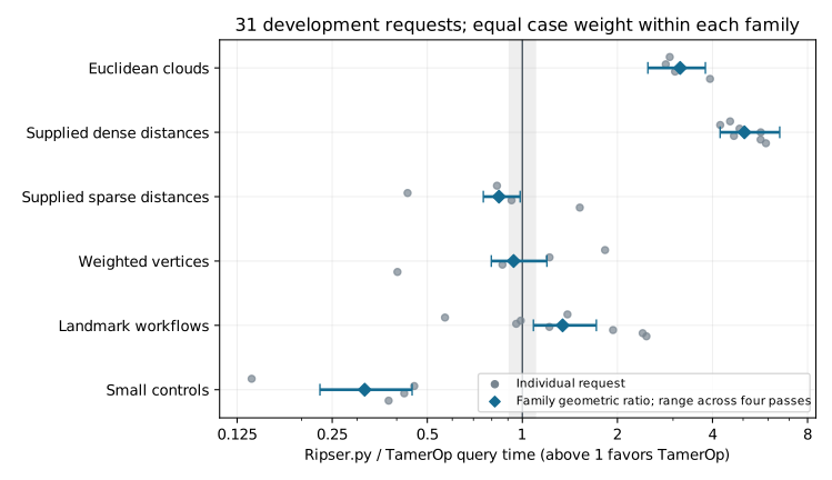
Gray points retain individual requests, including losses. Blue diamonds show family ratios; bars show paired-pass ranges. The shaded band marks practical similarity, not statistical equivalence. The horizontal scale is logarithmic. Full-size figure.
Development requests
Times are milliseconds; a degree label H₂ includes H₀, H₁ and H₂. Input size means points or vertices, with the selected landmark count shown separately. The interval count includes all returned degrees and essential bars, excluding zero-length intervals. Retained cocycles are computed inside the query timer.
| Request | Input size | Field / through | Cocycles | Intervals | TamerOp (ms) | Ripser.py (ms) | Ripser/TamerOp |
|---|---|---|---|---|---|---|---|
| Circle (point cloud) | 96 | F2 / H1 | No | 97 | 5.81 | 20 | 2.93 |
| Sphere (point cloud) | 64 | F3 / H2 | Yes | 81 | 13.8 | 41.8 | 2.84 |
| Sphere (point cloud) | 128 | F101 / H2 | No | 166 | 156 | 530 | 3.04 |
| Circle (distances) | 1,024 | F2 / H1 | No | 1025 | 7,010 | 30,400 | 4.55 |
| Sphere (distances) | 96 | F3 / H2 | Yes | 128 | 39.6 | 162 | 4.23 |
| Planar points (distances) | 128 | F101 / H2 | No | 154 | 29.3 | 133 | 4.87 |
| Grid graph | 256 | F2 / H1 | No | 481 | 0.469 | 0.341 | 0.831 |
| Cycle graph | 96 | F3 / H1 | Yes | 97 | 0.363 | 0.144 | 0.433 |
| Octahedral components | 96 | F101 / H2 | Yes | 112 | 0.598 | 0.499 | 0.924 |
| Grid graph (weighted vertices) | 256 | F2 / H1 | Yes | 481 | 0.794 | 1.26 | 1.83 |
| Grid graph (weighted vertices) | 4,096 | F2 / H1 | No | 8065 | 4.16 | 4.15 | 1.22 |
| Octahedral components (weighted vertices) | 96 | F101 / H2 | Yes | 112 | 0.658 | 0.51 | 0.865 |
| Greedy landmarks | 256 / 32 landmarks | F2 / H1 | No | 41 | 0.546 | 0.721 | 1.39 |
| Greedy landmarks | 2,048 / 128 landmarks | F2 / H1 | No | 186 | 13.9 | 7.66 | 0.569 |
| Greedy landmarks | 256 / 64 landmarks | F3 / H1 | Yes | 89 | 2.28 | 2.35 | 0.988 |
| Greedy landmarks | 512 / 96 landmarks | F101 / H1 | Yes | 136 | 5.29 | 5.03 | 0.956 |
| 3-sphere control | 8 | F2 / H3 | No | 9 | 1.45 | 0.188 | 0.139 |
| Octahedral components | 6 | F3 / H2 | Yes | 7 | 0.313 | 0.128 | 0.455 |
| Equal-grade control | 8 | F101 / H2 | Yes | 8 | 0.31 | 0.121 | 0.423 |
| Stored-zero cycle | 6 | F2 / H1 | Yes | 5 | 0.262 | 0.097 | 0.377 |
| Planar points (distances) | 512 | F101 / H2 | No | 643 | 2,150 | 11,700 | 5.69 |
| Greedy landmarks | 4,096 / 512 landmarks | F2 / H1 | No | 766 | 133 | 155 | 1.22 |
| Greedy landmarks | 4,096 / 1,024 landmarks | F2 / H1 | No | 1548 | 346 | 618 | 1.94 |
| Greedy landmarks | 4,096 / 3,072 landmarks | F2 / H1 | No | 4426 | 3,020 | 6,790 | 2.4 |
| Circle (point cloud) | 512 | F2 / H1 | Yes | 513 | 643 | 2,850 | 3.93 |
| Circle (distances) | 256 | F2 / H1 | No | 257 | 59.4 | 304 | 4.68 |
| Grid graph | 4,096 | F2 / H1 | No | 8065 | 2.66 | 4.07 | 1.52 |
| Cycle graph (weighted vertices) | 96 | F3 / H1 | Yes | 97 | 0.371 | 0.145 | 0.402 |
| Planar points (distances) | 256 | F101 / H2 | No | 313 | 189 | 1,130 | 5.68 |
| Planar points (distances) | 384 | F101 / H2 | No | 477 | 663 | 4,400 | 5.91 |
| Greedy landmarks | 4,096 / 2,048 landmarks | F2 / H1 | No | 3071 | 1,160 | 3,070 | 2.47 |
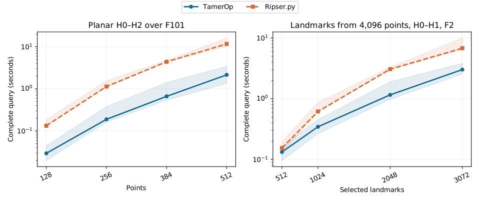
Bands show the range of four process medians. Lines connect the declared instances; they do not predict unmeasured sizes. The planar instances also differ in geometry. The landmark sequence uses the same 4,096-point metric. Vertical scales are logarithmic to keep both short and long requests visible. Full-size figure.
The small-subset landmark request takes 13.9 ms versus 7.66 ms at 2,048 points and 128 landmarks. The 3,072-landmark request takes 3.02 s versus 6.79 s. TamerOp validates the complete supplied distance matrix and retains its normal public outputs. Both implementations use farthest-point selection. These different outcomes should not be reduced to a single claim about all landmark workflows. Small sparse, weighted and algebraic controls likewise retain their measured relative losses even where the absolute delay is below a millisecond.
Reserved evaluation cases
These six recipes were reserved before optimization and first generated after the candidate was frozen. They include a jittered circle, new planar and spherical samples, relabeled grid and octahedral graphs, and a new dyadic landmark metric. No code was tuned after seeing their outcomes. Relabeling tests sensitivity to vertex order; it does not introduce a new module type. They are a small separate generalization check, not evidence about all inputs.
| Request | Input size | Field / through | Cocycles | Intervals | TamerOp (ms) | Ripser.py (ms) | Ripser/TamerOp |
|---|---|---|---|---|---|---|---|
| Jittered circle (point cloud) | 512 | F2 / H1 | Yes | 513 | 854 | 3,510 | 4.13 |
| Random planar (distances) | 128 | F101 / H2 | No | 159 | 25.4 | 127 | 4.83 |
| Random sphere (distances) | 96 | F3 / H2 | Yes | 124 | 49.7 | 186 | 3.81 |
| Permuted grid | 4,096 | F2 / H1 | No | 8065 | 4.19 | 7.69 | 1.85 |
| Permuted octahedra (weighted vertices) | 96 | F101 / H2 | Yes | 112 | 0.747 | 0.621 | 0.832 |
| Greedy landmarks | 2,048 / 128 landmarks | F2 / H1 | No | 187 | 15.7 | 7.9 | 0.546 |
Correctness and remaining limits
All 148 paired case/pass checks passed. Supplied grades are exactly Float32-representable, so complete interval multisets agree exactly. Native Euclidean clouds form a separate numerical lane: TamerOp uses Float64 distances, while Ripser.py converts filtration grades to Float32. Endpoints are compared at eight Float32 epsilons times their scale; possibly collapsed tiny bars are counted explicitly in the downloadable verification record.
Independent checks reconstruct landmark choices, retained tables and covering radii. Small controls use oriented boundary reduction; graph families use independent formulas or componentwise reduction. Every accepted computation matches its process's first complete mathematical export, covering all bars, requested landmark metadata and the selected witness cochains.
The verifier checks up to six longest positive-degree cocycles per degree. All 520 sampled witness checks establish closure and nontriviality, with restriction to an earlier scale where applicable. For large connected H₂ examples, a separate exact sparse linear-system test proves that the sampled cochain is not a coboundary. This closes the earlier sampled nontriviality gap; it does not certify every returned cochain or identify all large-output bases across tools. Small controls also compare complete class spaces.
The frozen mathematical implementation matches the one that passed 1,147,270 focused Rips, A115 and A117 assertions. Its only subsequent source difference is a visualization builder outside these calls. That owner-level evidence and the final cross-tool checks are not a claim that the entire package test suite was rerun. The strengthened verifier also passes its independent test set.
Machine and versions
| Item | Configuration |
|---|---|
| Processor | 13th Gen Intel(R) Core(TM) i7-1365U; 10 physical cores / 12 logical CPUs |
| RAM | 31.00 GiB OS-visible |
| System | Linux-6.8.0-138-generic-x86_64-with-glibc2.35 |
| Julia | 1.12.1 |
| Python | 3.12.3 |
| Comparator | Ripser.py 0.6.15, Robin Hood 3.11.5, -O3 |
| Execution | One numerical thread; serial workers pinned to logical CPU 0 |
| Limits | 7 GiB worker RSS; 180 s per phase; 420 s startup; 3,600 s per worker |
| Host activity | One-minute load min/median/max: 1.29 / 4.12 / 7.02 |
No worker hit a time or memory limit. Completed workers took about 53.5 minutes in total, including loading, compilation, warmup, input decoding, output checks and compression. That duration is not the time spent on the mathematical requests alone. The machine was not exclusively reserved; monitored activity and run-to-run variation remain part of the evidence.
This uses Ripser.py's supported optimized source build, not a search over all compiler configurations. Its extension hash was checked before launch. TamerOp is the frozen development source listed in the downloadable hashes, including unreleased improvements; a version number or Git commit alone does not identify this working-tree snapshot. Existing package-cache flags were used for loading, so first-use records are diagnostic and do not measure a normal freshly installed package's startup.
Allocations and memory
Julia allocation traffic, native retained-output estimates, current process RSS and process high-water RSS are distinct measurements. The downloads keep them separate. Python allocation traffic is unmeasured; it must not be treated as zero. Neither runtime's retained-output estimate is an exact measure of mathematical storage. Full-process RSS includes runtime and compiled code, inputs, working memory and allocations retained by the allocator.
The largest monitored worker RSS was 3.09 GiB. Per-case Julia allocations and per-tool RSS/output estimates are in the CSV. No memory-based speed ranking is substituted for elapsed computation time.
Data and reproduction
- All case times, sizes, allocations and memory estimates.
- Process medians, paired ratios and family summaries.
- Every accepted timed sample, rejected samples and first-use diagnostics.
- Mathematical verification and completion checks.
- Fixed manifest, reserved recipes, source hashes, harness hashes, comparator build and Python dependencies.
- Machine record, data notes and integrity checksums.
The public data support checking the tables and figures. The complete local archive also retains input files, frozen sources, worker scripts, compressed mathematical outputs and resource logs. That archive and the benchmark harness are intentionally excluded from Git; this download is not yet a portable bundle for rerunning the computations. A later reproduction release must include the inputs and pinned environments. No previous development times are pooled into this final study.
This closes the fixed Ripser.py v1 comparison. It establishes the reported workload-specific performance and correctness evidence; it does not assert that every possible optimization is exhausted or rank TamerOp's broader finite-encoding functionality against a Rips persistence engine.
The benchmarking manual explains the shared protocol. Comparator references: Ripser.py interface, supported source build, and Ripser algorithms.