From inputs to computed objects
Download the executed notebook · Build and environment record
All figures below are saved results; reading this page needs no Julia session. Select a figure to view it at full size.
What can I start with, and what can I do with the result? A familiar filtration and a module described directly by regions can both lead to a finite encoding. We will construct one of each, recover a space and a map, and perform the same algebraic operation on both finite modules.
The first example starts with two points and two filtration parameters. The second starts with a sloped strip in the parameter plane. The objects are different; the finite-module queries let us ask the same kinds of questions about them.
You need basic vector spaces, matrices, and coordinatewise comparison of pairs. Persistence modules explains those ideas, and finite encodings explains the retained object. To run the guide, use Julia 1.12 with TamerOp and CairoMakie in the documented notebook environment. No input files are needed. The saved figures can also be read without Julia.
| What you already have | Where to begin | What you obtain |
|---|---|---|
| Points, images, graphs, or cells with filtration grades | A supported filtration and its encoding workflow | An encoding of the selected persistence module, with its parameter assignment |
| Supported geometric upsets and downsets, with a coefficient matrix | An indicator presentation | An encoding of the module specified by that presentation |
| A finite poset with compatible spaces and maps | A finite PModule | A module already in the finite setting; parameter lookup is unnecessary |
For a direct one-parameter barcode computation, the ordinary-persistence guide provides a shorter route. Such a call need not construct an encoding. Here we retain a module because we want to ask further questions about its maps and algebra.
Set up the two computations
OP provides the main workflows. OA exposes the detailed region, module, and morphism constructors used below. We choose the rational field for vector spaces and matrices, and CairoMakie for saved static figures.
import TamerOp as OP
import TamerOp.Advanced as OA
import TamerOp.CoreModules: QQField
import LinearAlgebra: I
import CairoMakie
CairoMakie.activate!(type="png", px_per_unit=1)
field = QQField();
Start from a filtration
Take two points at $(0,0)$ and $(3,4)$, whose distance is 5. Give them function values 0 and 1. A function–Rips filtration uses two increasing parameters: an edge-length threshold $r$ and a function threshold $a$. A vertex is present when its function value is at most $a$; an edge is present when both endpoints are present and their distance is at most $r$.
Thus the second point enters at $a=1$, and the edge connecting the points enters at $r=5$. Here $r$ is an edge-length threshold, not the radius of balls around the points. We retain vertices and edges (max_dim=1), which suffice to determine connected components.
points = OP.PointCloud([[0.0, 0.0], [3.0, 4.0]])
filtration = OP.FunctionRipsFiltration(
    vertex_values=[0.0, 1.0], max_dim=1);
OP.visualize(points; kind=:points_2d, labels=["u", "v"])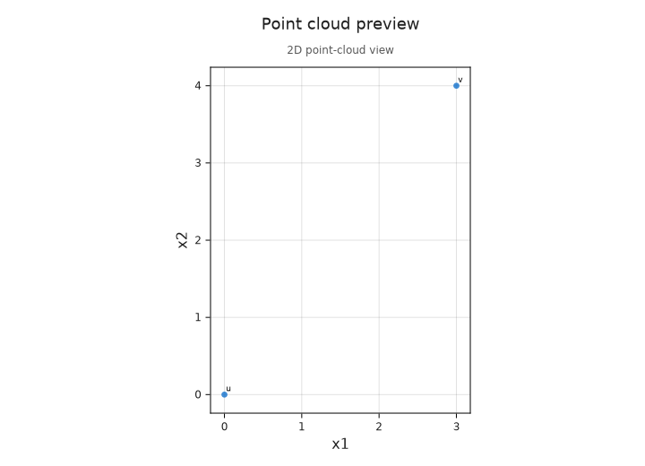
The picture shows the physical point coordinates. The filtration parameters $(r,a)$ form a different plane: distance controls the edge, while the supplied function controls vertex appearance.
We can predict degree-zero homology before calling the library. Each connected component contributes one independent vector.
| Parameter $(r,a)$ | Present cells | Number of components |
|---|---|---|
| $(1/2,0)$ | First vertex | 1 |
| $(1/2,1)$ | Both vertices, no edge | 2 |
| $(5,1)$ | Both vertices and their edge | 1 |
The final step merges the two components. Its map has a two-dimensional source, a one-dimensional target, and rank one.
data_encoding = OP.encode(points, filtration; degree=0, field=field)
OP.describe(data_encoding)
(kind = :encoding_result, poset_type = TamerOp.FiniteFringe.ProductOfChainsPoset{2}, module_type = TamerOp.DataIngestion._LazyEncodedModule, encoding_map_type = TamerOp.EncodingCore.CompiledEncoding{TamerOp.EncodingCore.GridEncodingMap{2, Float64, TamerOp.FiniteFringe.ProductOfChainsPoset{2}}, TamerOp.FiniteFringe.ProductOfChainsPoset{2}, Nothing, Nothing, @NamedTuple{encoding_cache::TamerOp.CoreModules.EncodingCache}}, compiled = true, backend = :data, has_cohomology = false, has_presentation = true, module_dims = nothing, materialized = false, provenance = (category = :finite_poset_representations, base_poset = ProductOfChainsPoset(axes=(2, 2), nvertices=4), field = QQField(), degree = 0, degree_convention = :homological, encoding = (map_type = TamerOp.EncodingCore.CompiledEncoding{TamerOp.EncodingCore.GridEncodingMap{2, Float64, TamerOp.FiniteFringe.ProductOfChainsPoset{2}}, TamerOp.FiniteFringe.ProductOfChainsPoset{2}, Nothing, Nothing, @NamedTuple{encoding_cache::TamerOp.CoreModules.EncodingCache}}, backend = :data), window = (lower = (0.0, 0.0), upper = (5.0, 1.0), coordinates = :oriented, outside_lower = :unrepresented, upper_extension = :constant), orientation = (1, 1), construction = (requested = :function_rips, effective = :function_rips, substitution = :none, projection = :none, grade_scale = :diameter, requested_max_dim = 1, retained_max_dim = 1), discretization = (axes_policy = :encoding, axes_source = :computed_grades, axis_kind = nothing, grade_placement = :critical_grades, sampling = false, quantization = :none, eps = nothing), approximation = (sparsify = :none, input_point_count = 2, retained_vertex_count = 2, radius_cutoff = nothing, collapse = :none, multicritical = :union, onecritical_selector = nothing, onecritical_enforce_boundary = nothing, grade_arithmetic = :float64, neighbor_search = :not_used, construction_substitution = :none), backend = (requested = (ingestion = :data, neighbors = :auto, multicover = :auto, delaunay = :auto), effective = :native, linear_algebra = :operation_specific), ambient_identification = :not_asserted, chain_storage = :cochain_reindexed_homology, reconstruction = :computed_graded_complex))This EncodingResult retains a finite poset and an assignment from filtration parameters to its labels. Its spaces and maps may be deferred until requested. encoding_module requests the finite module; the same accessor works for the region example below.
Here we inspect the domain r ≥ 0, a ≥ 0. The default grid includes the critical grades. Selecting a coarser grid can change the represented module; ingestion choices explains that distinction. A grid lookup below its first grade can return the unrepresented-label sentinel 0, which is different from a represented zero space.
data_module = OP.encoding_module(data_encoding)
data_classifier = OP.encoding_map(data_encoding)
data_dimensions = OP.dimensions(data_encoding)
parameters = [(1//2, 0//1), (1//2, 1//1), (5//1, 1//1)]
labels = [OA.locate(data_classifier, p) for p in parameters]
@assert all(>(0), labels)
@assert data_dimensions[labels] == [1, 2, 1]
(; parameters, dimensions=data_dimensions[labels])
(parameters = Tuple{Rational{Int64}, Rational{Int64}}[(1//2, 0), (1//2, 1), (5, 1)], dimensions = [1, 2, 1])A parameter chooses a finite label; that label chooses a space. These labels belong to the returned encoding, so we obtain them by lookup instead of guessing their numeric IDs.
Now recover the merge map. structure_map takes finite labels. The original parameters are comparable in coordinatewise order, which justifies this query as a map in the persistence module.
merge_map = OA.structure_map(data_module;
    source=labels[2], target=labels[3])
@assert merge_map == OP.QQ[1 1]
merge_map
1×2 TamerOp.DataIngestion._StructuralInclusionMap{Rational{BigInt}}:
1 1The row $[1\;1]$ sends the two component coordinates $(u,v)$ to $u+v$: both source components become the same connected component. Its kernel is the line of differences $(v,-v)$.
The inspector links the selected parameters, their finite labels, and the matrix. In its parameter panel, the first coordinate is $r$ and the second is $a$. The viewing window controls the drawing; it does not change the encoded module.
data_window = ([0.0, 0.0], [7.0, 3.0])
OP.visualize(data_encoding; kind=:module_inspector,
    parameter_pair=(parameters[2], parameters[3]), box=data_window)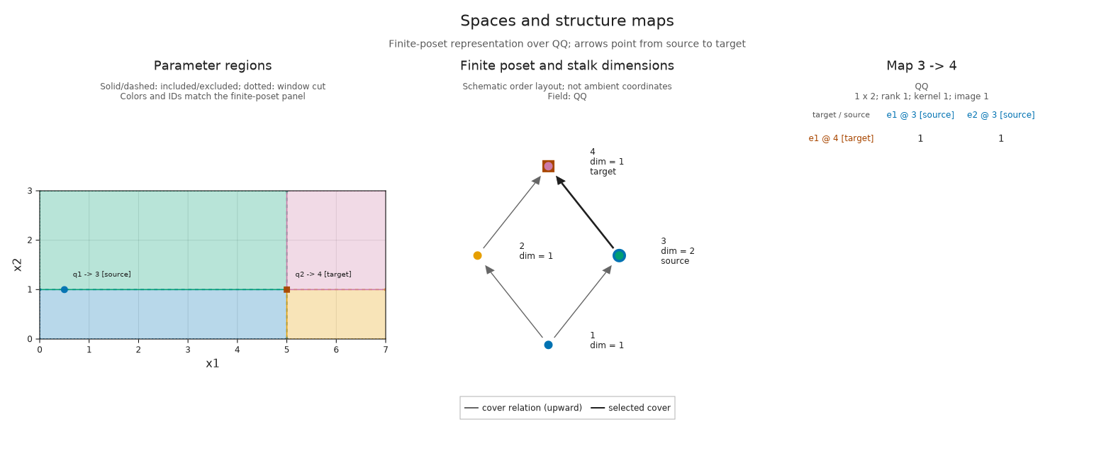
We can also ask for a numerical invariant. The rank invariant records the rank of each comparable-pair map. It keeps those numbers, while the encoding remains available for matrix queries and further algebra.
data_ranks = OP.invariant(data_encoding; which=:rank_invariant)
merge_rank = OA.value_at(OP.invariant_value(data_ranks), labels[2], labels[3])
@assert merge_rank == 1
merge_rank1Define a module by regions
We can specify a persistence module without supplying a point cloud or a filtration. Consider the closed strip
\[S=\{(x,y)\in\mathbb R^2:0\leq x+y\leq1\}.\]
At a point of $S$, assign the space $\mathbb Q$; elsewhere assign zero. Between comparable points inside $S$, use the identity map. All other prescribed maps are zero. Any point between two comparable points of the strip remains in the strip. This order-convexity condition makes the prescribed maps compose consistently.
This support has sloped boundaries and extends without bound in the direction $(1,-1)$. A finite axis-aligned grid of critical coordinates cannot describe those boundaries exactly throughout the original plane. A finite region encoding can: it distinguishes below the strip, inside it, and above it.
Write $S=U\cap D$, where the upset $U$ satisfies $x+y\geq0$ and the downset $D$ satisfies $x+y\leq1$. Increasing coordinates keeps a point in the upset; decreasing them keeps a point in the downset. make_hpoly(A,b) describes the inequalities $Az\leq b$. Thus the first inequality uses the row $[-1\;-1]$, and the second uses $[1\;1]$.
U = OA.PLUpset(OA.poly_union(
    OA.make_hpoly(OP.QQ[-1 -1], OP.QQ[0])))
D = OA.PLDownset(OA.poly_union(
    OA.make_hpoly(OP.QQ[1 1], OP.QQ[1])))
presentation = OA.PLFringe([U], [D], reshape(OP.QQ[1], 1, 1));
The coefficient $[1]$ defines the map from the upset indicator to the downset indicator. Its image is one-dimensional exactly where both regions are active. That image is our strip module; indicator presentations explains the construction more generally.
Select the general polyhedral encoder for the sloped regions. The rational inequality coefficients retain the exact boundary geometry. The field option separately specifies rational arithmetic in the vector spaces.
strip_encoding = OP.encode(presentation,
    OA.EncodingOptions(backend=:pl, field=field))
strip_module = OP.encoding_module(strip_encoding)
strip_classifier = OP.encoding_map(strip_encoding)
strip_dimensions = OP.dimensions(strip_encoding)
@assert OA.nvertices(OP.encoding_poset(strip_encoding)) == 3
@assert sort(strip_dimensions) == [0, 0, 1]
(; finite_labels=length(strip_dimensions), dimensions=strip_dimensions)
(finite_labels = 3, dimensions = [0, 1, 0])The whole plane is represented with three labels, including the two zero regions. A zero space outside the strip is part of the module, not missing information.
Choose $s=(0,0)$ and $t=(1/4,1/4)$. Both lie in the strip, and $s\leq t$, so the expected map is $[1]$. The boundary point $(1,0)$ is also included. Finally, $(100,-100)$ lies on the lower boundary: the construction is not confined to the plotted window.
s, t = (0//1, 0//1), (1//4, 1//4)
qs, qt = [OA.locate(strip_classifier, p) for p in (s, t)]
strip_map = OA.structure_map(strip_module; source=qs, target=qt)
@assert strip_map == reshape(OP.QQ[1], 1, 1)
@assert strip_dimensions[OA.locate(strip_classifier, (1, 0))] == 1
@assert strip_dimensions[OA.locate(strip_classifier, (100, -100))] == 1
strip_map
1×1 Matrix{Rational{BigInt}}:
1strip_window = ([-1.0, -1.0], [2.0, 2.0])
OP.visualize(strip_encoding; kind=:module_inspector,
parameter_pair=(s, t), box=strip_window)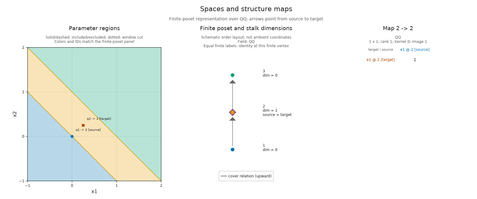
The sloped region in the parameter panel is the nonzero support. The finite model has a three-element chain, with a one-dimensional space at the middle label. Its two cover maps are zero, since one endpoint is a zero space; their composite is zero as well. The selected map is the identity at the middle label.
The mathematical boundary tests above use exact rational data. Rendering those regions on a screen uses finite drawing precision. The window cuts off the picture, not the strip.
Change the target and predict the answer
Move the target to $z=(1,1)$. The pair $s\leq z$ is still comparable, but $z$ lies above the strip. Predict the matrix shape and rank. Then compare the same rank-invariant query used for the filtration.
z = (1, 1)
qz = OA.locate(strip_classifier, z)
leaving_map = OA.structure_map(strip_module; source=qs, target=qz)
strip_ranks = OP.invariant(strip_encoding; which=:rank_invariant)
leaving_rank = OA.value_at(OP.invariant_value(strip_ranks), qs, qz)
@assert size(leaving_map) == (0, 1)
@assert leaving_rank == 0
(; matrix_size=size(leaving_map), rank=leaving_rank)
(matrix_size = (0, 1), rank = 0)OP.visualize(strip_encoding; kind=:module_inspector,
parameter_pair=(s, z), box=strip_window)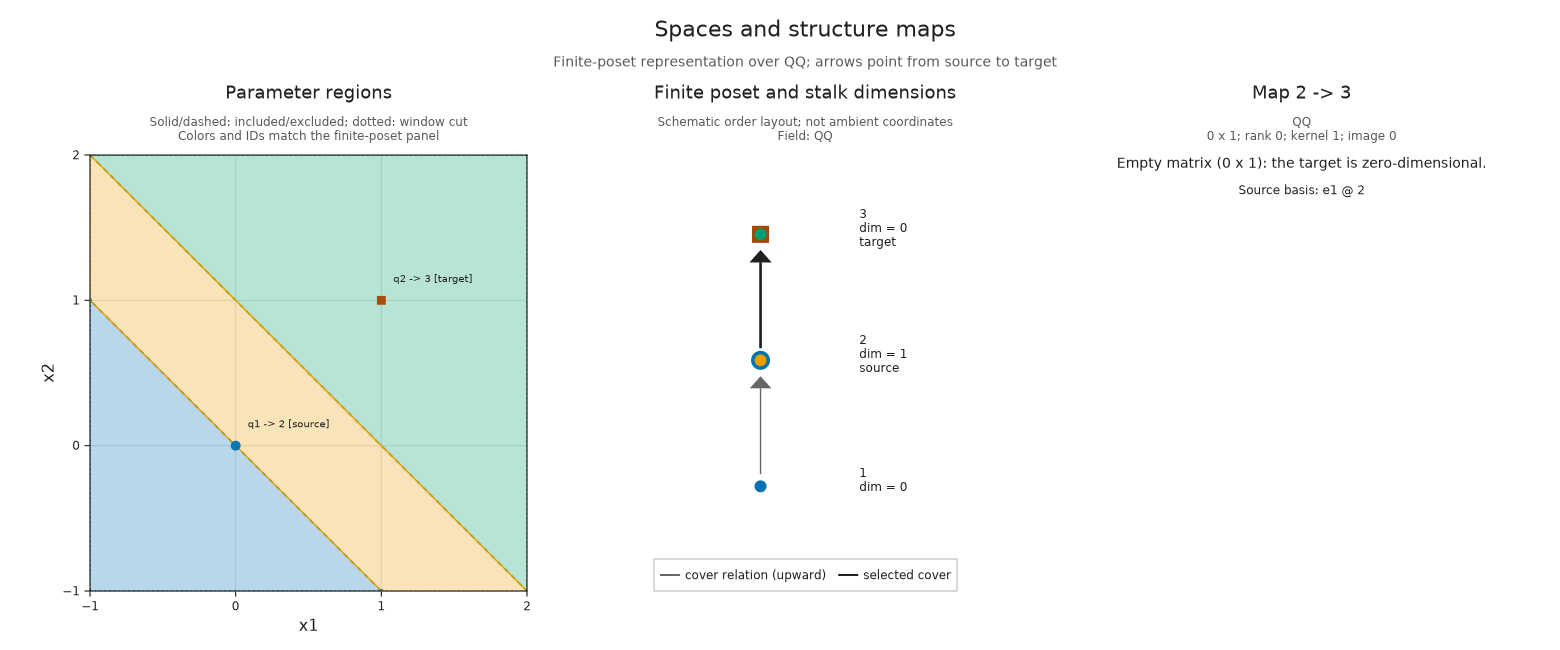
A zero map is different from the absence of a map. For example, (0,1) and (1,0) are both in the strip but incomparable. Sharing a finite label does not supply a structure map between incomparable original parameters. The spaces-and-maps guide explains parameter-aware inspection and this distinction in more detail.
Continue with algebra on either module
The filtration route has not used up its module by producing a rank. Both data_module and strip_module retain spaces and compatible maps, so both can participate in finite-poset algebra.
Here is a module morphism with a known answer. Take two copies of a module $M$ and add their vectors at each label:
\[\alpha:M\oplus M\longrightarrow M,\qquad \alpha_p(u,v)=u+v.\]
If a structure map of $M$ is $A$, then $A(u+v)=Au+Av$. Thus addition commutes with every structure map. This compatibility makes the family of matrices $[I\;I]$ a module morphism, as opposed to a structure map between two spaces within one module.
Its kernel at each label consists of pairs $(u,-u)$. These spaces fit together into a kernel module isomorphic to $M$. This prediction applies independently to the data-derived module and the strip module; their finite base posets need not agree with each other.
data_double = OA.direct_sum(data_module, data_module)
data_addition = OA.PMorphism(data_double, data_module,
    [hcat(Matrix{OP.QQ}(I, d, d), Matrix{OP.QQ}(I, d, d))
     for d in data_dimensions])
@assert OA.check_morphism(data_addition).valid
data_kernel, data_inclusion = OA.kernel_with_inclusion(data_addition)
@assert OP.dimensions(data_kernel).stalks == data_dimensions
OP.dimensions(data_kernel)
(vertices = 4, stalks = [1, 1, 2, 1], total = 5, maximum_stalk = 2, edges = 4)kernel_with_inclusion returns both the kernel module and its inclusion into the doubled module. Returning that inclusion matters: it tells us how the computed vectors sit inside the original coordinates.
At the two-component label, addition maps four coordinates to two. Check that the inclusion's columns are killed by addition and that inclusion commutes with the merge map. These are checks of actual maps, beyond agreement of dimensions.
First inspect the addition matrix at that label.
p, q = labels[2], labels[3]
addition_at_p = OA.component(data_addition, p)
inclusion_at_p = OA.component(data_inclusion, p)
inclusion_at_q = OA.component(data_inclusion, q)
kernel_merge = OA.structure_map(data_kernel; source=p, target=q)
doubled_merge = OA.structure_map(data_double; source=p, target=q)
@assert addition_at_p * inclusion_at_p == zeros(OP.QQ, 2, 2)
@assert doubled_merge * inclusion_at_p == inclusion_at_q * kernel_merge
addition_at_p
2×4 Matrix{Rational{BigInt}}:
1 0 1 0
0 1 0 1The inclusion has one column for each kernel coordinate. Its four rows give the coordinates in the doubled two-component space.
inclusion_at_p4×2 Matrix{Rational{BigInt}}:
0 -1
-1 0
0 1
1 0The kernel module also has its own merge map from $p$ to $q$:
kernel_merge1×2 Matrix{Rational{BigInt}}:
1 1The equality being checked is the commutative square
\[\begin{array}{ccc} K(p)&\xrightarrow{\ \iota_p\ }&(M\oplus M)(p)\\ {\scriptstyle K(p\leq q)}\downarrow&&\downarrow{\scriptstyle (M\oplus M)(p\leq q)}\\ K(q)&\xrightarrow{\ \iota_q\ }&(M\oplus M)(q). \end{array}\]
In words, include a kernel vector and then move along the filtration, or first move in the kernel module and then include it: both paths give the same vector. The software chooses bases for these kernel spaces, so their inclusion matrices need not use our preferred signs.
Repeat the construction for the strip using the same public operations. Display its kernel inclusion at the selected label inside the strip.
strip_double = OA.direct_sum(strip_module, strip_module)
strip_addition = OA.PMorphism(strip_double, strip_module,
    [hcat(Matrix{OP.QQ}(I, d, d), Matrix{OP.QQ}(I, d, d))
     for d in strip_dimensions])
@assert OA.check_morphism(strip_addition).valid
strip_kernel, strip_inclusion = OA.kernel_with_inclusion(strip_addition)
@assert OP.dimensions(strip_kernel).stalks == strip_dimensions
@assert OA.component(strip_addition, qs) * OA.component(strip_inclusion, qs) == zeros(OP.QQ, 1, 1)
OA.component(strip_inclusion, qs)
2×1 Matrix{Rational{BigInt}}:
-1
1Inside the strip, two coordinates add to one and their one-dimensional difference space forms the kernel. Outside, all of these spaces are zero. The kernel is again a finite module; the original strip classifier supplies its interpretation on the plane.
The addition construction works for an already supplied PModule as well. Each morphism must have source and target on the same finite base and over the same field. Comparing separately constructed geometric encodings requires a justified common base; it is not enough to match their numeric label IDs.
Resolutions, Ext, Tor, and products provide further questions on finite modules. Their results belong to the actual finite-poset category being computed in. Recovery of an ambient module does not by itself make finite-category Ext or Tor independent of the encoding. The category guide states those contracts.
Choose the next question
The two routes supplied different persistence modules, but both supported parameter lookup, matrix queries, a rank invariant, and a kernel construction. The geometric route retained a sloped support exactly; the filtration route retained the maps induced by its cells. A summary can answer one question without preventing further work with the encoding.
Continue with exploring spaces and maps to choose more queries and coordinate views. For the mathematics behind the directly specified input, read indicator presentations.