Inspect spaces and maps
Download the executed notebook · Build and environment record
All figures below are saved results; reading this page needs no Julia session. Select a figure to view it at full size.
How does a finite encoding recover a space and a map at the parameters we choose? We will construct the closed square from finite encodings, follow points into its finite model, and read the answer in matrices and figures. Then two overlapping squares will show why knowing the dimensions is not enough.
You need coordinatewise order on pairs and basic matrix multiplication. The two-parameter introduction supplies the first idea; persistence modules gives the fuller definitions. No input files are needed. To run the cells, use Julia 1.12 with TamerOp and CairoMakie; the installation guide explains the setup. You can also read the saved figures without running Julia.
Our route is to predict the square's spaces, construct its encoding, recover selected maps, and change the example. Presentation coordinates, live exploration, and export are optional sections at the end.
Predict the square before computing
At a parameter $q=(q_1,q_2)$, our module assigns the vector space $\mathbb Q$ if both coordinates lie between 0 and 2, and the zero space otherwise. The region where the space is nonzero is its support, the closed square $S=[0,2]^2$. The module is defined on the whole real plane, including outside this square.
For comparable parameters $q\leq r$, the map is the identity if both points lie in $S$, and zero otherwise. Here are three predictions. A matrix has one row for each target coordinate and one column for each source coordinate.
| Parameters | Spaces | Expected matrix |
|---|---|---|
| $(1/2,1/2)\leq(3/2,3/2)$ | $\mathbb Q\longrightarrow\mathbb Q$ | The $1\times1$ matrix $[1]$ |
| $(1/2,1/2)\leq(3,1)$ | $\mathbb Q\longrightarrow0$ | An empty matrix of size $0\times1$ |
| $(1/4,3/2)$ and $(3/2,1/4)$ | Both spaces are $\mathbb Q$ | No structure map: the points are incomparable |
All four edges belong to the square. In particular, $(0,0)$ and $(2,2)$ have one-dimensional spaces. The rational coefficient field $\mathbb Q$ describes vectors and matrices; it does not restrict the parameter plane to rational points. We are specifying this module directly, not deriving it from the earlier ring's filtration.
Describe the support with two regions
Import TamerOp as OP and load CairoMakie for static figures. We also import Advanced as OA for region constructors and detailed algebraic queries. The main construction still uses the public OP.encode workflow. Selecting PNG display lets the notebook retain the figures.
import TamerOp as OP
import TamerOp.Advanced as OA
import TamerOp.CoreModules: QQField
import CairoMakie
CairoMakie.activate!(type="png", px_per_unit=1);
Let $U$ contain all points above $(0,0)$, and let $D$ contain all points below $(2,2)$. Their intersection is our square. BoxUpset describes $U$, which is closed under increasing coordinates; BoxDownset describes $D$, which is closed under decreasing them. Neither region is a bounded box.
We supply one coefficient, the $1\times1$ matrix $[1]$. At a parameter in both regions this gives the map $\mathbb Q\to\mathbb Q$ with image $\mathbb Q$. Elsewhere its image is zero. Thus the image of this small indicator presentation is precisely our square module. The presentation chapter develops the general construction; this one coefficient is all we need here.
births = [OA.BoxUpset([0, 0])]
deaths = [OA.BoxDownset([2, 2])]
coefficient = reshape(OP.QQ[1], 1, 1)
1×1 Matrix{Rational{BigInt}}:
1We choose rational arithmetic for the vector spaces and a signature encoding for these geometric regions. A signature records which input supports are active. These are mathematical representation choices, so we state them explicitly. The box constructor stores its corners in floating-point coordinates; the integer corners used here are exactly representable.
field = QQField()
options = OA.EncodingOptions(; backend=:pl_backend,
    poset_kind=:signature, field=field);
encode returns an EncodingResult. It keeps the finite poset, the assignment from original parameters to its labels, and the encoded module together. The object is useful because a query on the plane can be answered using that finite information.
enc = OP.encode(births, deaths, coefficient, options);Read the finite object we actually received
Use the semantic accessors to obtain the poset P, the parameter-to-label map classifier, and the vector of stalk dimensions. Entry dims[q] is the dimension at finite label q. A stalk is the vector space at a parameter or a finite label.
P = OP.encoding_poset(enc)
classifier = OP.encoding_map(enc)
dims = OP.dimensions(enc)
@assert OP.provenance(enc).field == field
@assert OA.nvertices(P) == 4
@assert sort(dims) == [0, 0, 0, 1]
(; nvertices=OA.nvertices(P), dimensions=dims)
(nvertices = 4, dimensions = [0, 0, 1, 0])Why four labels, when the introductory chapter drew nine regions? The nine-region grid is one valid encoding. This encoder instead records two bits: whether a point belongs to $U$, and whether it lies outside $D$. Both bits can only increase as the original parameter increases.
| Signature | One parameter with this signature | Stalk dimension |
|---|---|---|
| $(0,0)$: outside $U$, inside $D$ | $(-1,-1)$ | 0 |
| $(1,0)$: inside $U$ and $D$ | $(1,1)$ | 1 |
| $(0,1)$: outside both $U$ and $D$ | $(-1,3)$ | 0 |
| $(1,1)$: inside $U$, outside $D$ | $(3,3)$ | 0 |
The numeric IDs belong to the returned object. locate discovers them; we do not assume that ID 1 means the first row of this table.
lower_id = OA.locate(classifier, (-1, -1))
inside_id = OA.locate(classifier, (1, 1))
mixed_id = OA.locate(classifier, (-1, 3))
upper_id = OA.locate(classifier, (3, 3))
@assert length(unique([lower_id, inside_id, mixed_id, upper_id])) == 4
@assert dims[[lower_id, inside_id, mixed_id, upper_id]] == [0, 1, 0, 0]
@assert OA.locate(classifier, (3, -1)) == mixed_id
(; lower_id, inside_id, mixed_id, upper_id)
(lower_id = 1, inside_id = 3, mixed_id = 2, upper_id = 4)First draw these labels in the parameter plane. kind chooses the view. box gives the lower-left and upper-right corners of the viewing window, not a restriction of the module. We will use this same window for every one-square comparison.
view_box = ([-1, -1], [5, 5])
OP.visualize(enc; kind=:region_labels, box=view_box)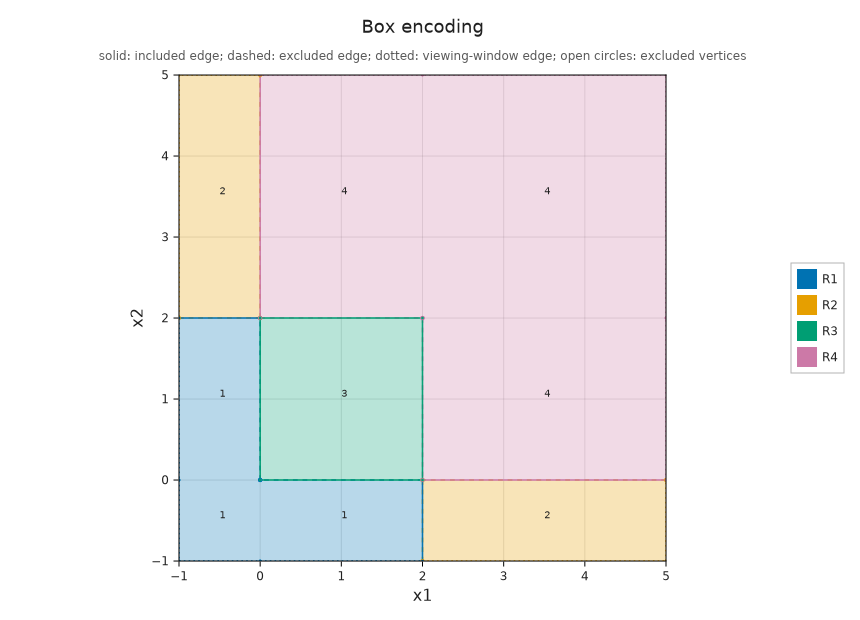
The closed central square has the label inside_id. Notice that the upper-left and lower-right exterior pieces share mixed_id. The set of points assigned one label is its fiber; it need not be connected. Colours identify finite labels; they do not count vectors. Solid and dashed boundaries distinguish included and excluded edges; dotted boundaries are cuts made by the viewing window.
Now draw the order on those labels. kind=:hasse shows a Hasse diagram: an arrow is a comparison with no label strictly in between. Upward means increasing in the finite order. The vertex positions are schematic, not coordinates from the parameter plane. Selecting vertex=inside_id highlights the square's label.
OP.visualize(enc; kind=:hasse, vertex=inside_id)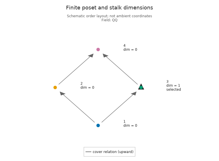
The two middle signatures $(1,0)$ and $(0,1)$ are incomparable. Their upper and lower neighbours give a diamond. Each vertex also records its stalk dimension. An arrow records an allowed comparison, not a claim that its linear map is nonzero. In this particular diamond every map between distinct labels is zero, because at least one endpoint space is zero.
The nine-label and four-label descriptions both recover the same square module. We are reading this returned representation, not claiming that four is the smallest possible encoding.
Follow a parameter to its space
Take $x=(1/2,1/2)$. The two steps are to find $\pi(x)$, its finite label, and then read $N(\pi(x))$, the space at that label in the finite module $N$. This is how the encoded module recovers $M(x)$.
Julia's 1//2 denotes an exact rational number. Here the chosen corners and query points are also exactly representable by the box geometry. Check the two corners as well as the interior: the square is closed.
x = (1//2, 1//2)
qx = OA.locate(classifier, x)
@assert qx == inside_id
@assert dims[qx] == 1
@assert OA.locate(classifier, (0, 0)) == inside_id
@assert OA.locate(classifier, (2, 2)) == inside_id
@assert OA.locate(classifier, (0, 2)) == inside_id
@assert OA.locate(classifier, (2, 0)) == inside_id
(; parameter=x, finite_label=qx, dimension=dims[qx])
(parameter = (1//2, 1//2), finite_label = 3, dimension = 1)The module inspector puts the recovery steps next to one another: the parameter picture, its finite poset, and the selected space. point=x selects an original parameter; vertex=qx would select a label directly.
OP.visualize(enc; kind=:module_inspector, point=x, box=view_box)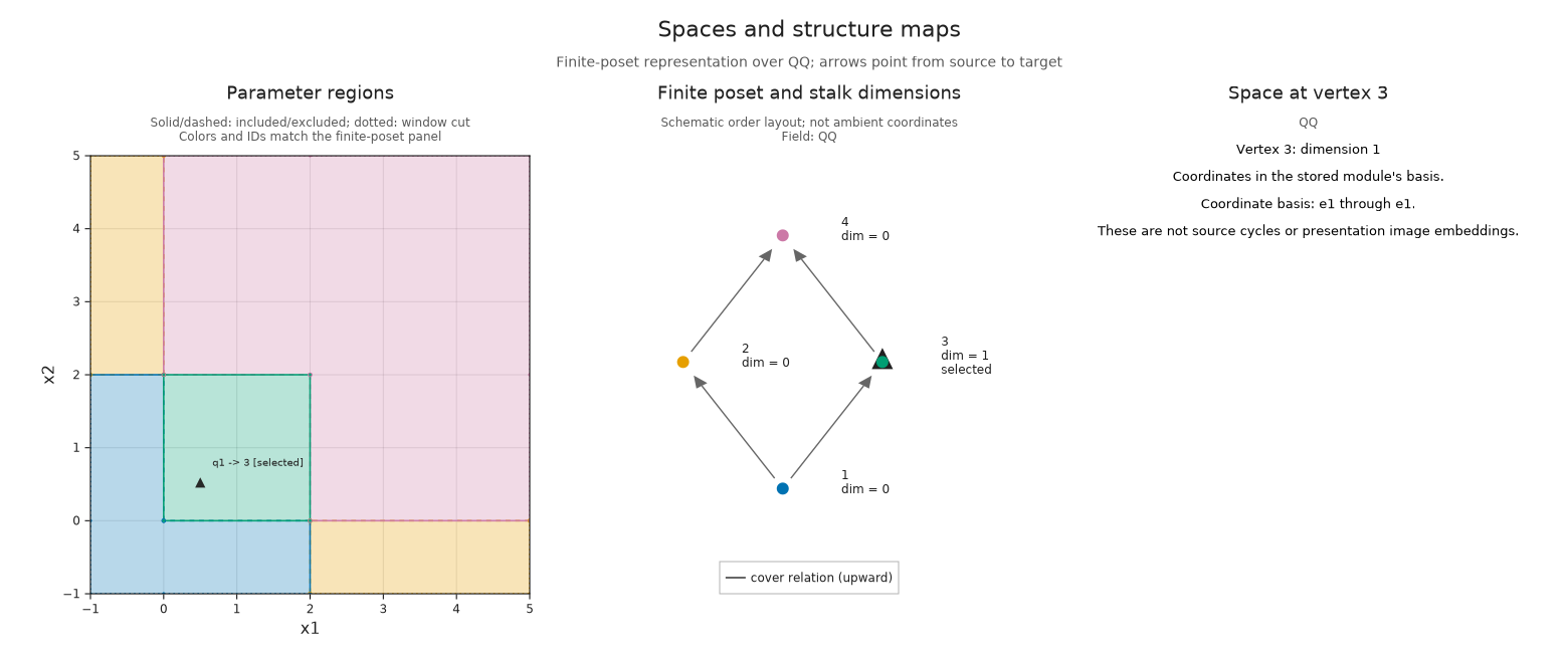
Read the panels from left to right. The marked point belongs to the highlighted label, whose space has dimension one. The colour and numeric ID link the two pictures. The readout concerns coordinates in the stored module; it does not name a geometric cycle from the earlier ring.
Recover a map between comparable parameters
Let $y=(3/2,3/2)$. Since $x\leq y$ coordinatewise, there is a structure map. Both points lie inside the square, so our prediction was the identity $[1]$.
encoding_module obtains the finite module and its maps. structure_map then takes finite labels, with the source and target named explicitly. We have checked the original comparison before making this finite query.
y = (3//2, 3//2)
qy = OA.locate(classifier, y)
square_module = OP.encoding_module(enc)
inside_map = OA.structure_map(square_module; source=qx, target=qy)
@assert inside_map == reshape(OP.QQ[1], 1, 1)
inside_map
1×1 Matrix{Rational{BigInt}}:
1For the figure, parameter_pair=(x,y) asks the inspector to retain the original parameters and check their order as well. The matrix's columns are source coordinates and its rows are target coordinates. Its rank, one, counts the independent vectors that survive this map.
OP.visualize(enc; kind=:module_inspector,
    parameter_pair=(x, y), box=view_box)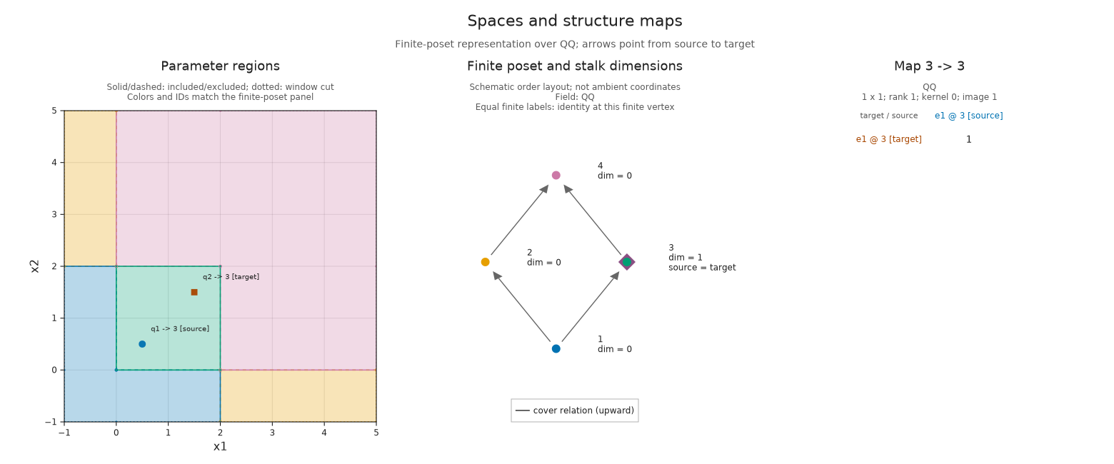
The parameter points are different, but their labels are the same. The map is therefore the identity at that label. A Hasse diagram omits identity arrows, so this nonzero continuation does not require an edge between two different vertices.
Exercise: a zero map or no map?
Move the target to $z=(3,1)$ and keep the source $x$. The pair remains ordered. Predict the target space, the matrix shape, and the rank before running the next cell.
z = (3, 1)
qz = OA.locate(classifier, z)
leaving_map = OA.structure_map(square_module; source=qx, target=qz)
@assert qz != 0 && dims[qz] == 0
@assert size(leaving_map) == (0, 1)
leaving_map
0×1 Matrix{Rational{BigInt}}The target is outside the support, so the map sends every vector to the zero space. Its matrix has zero rows and one column. There are no entries to draw, but the map is defined and its rank is zero. The figure reports that empty shape explicitly.
OP.visualize(enc; kind=:module_inspector,
    parameter_pair=(x, z), box=view_box)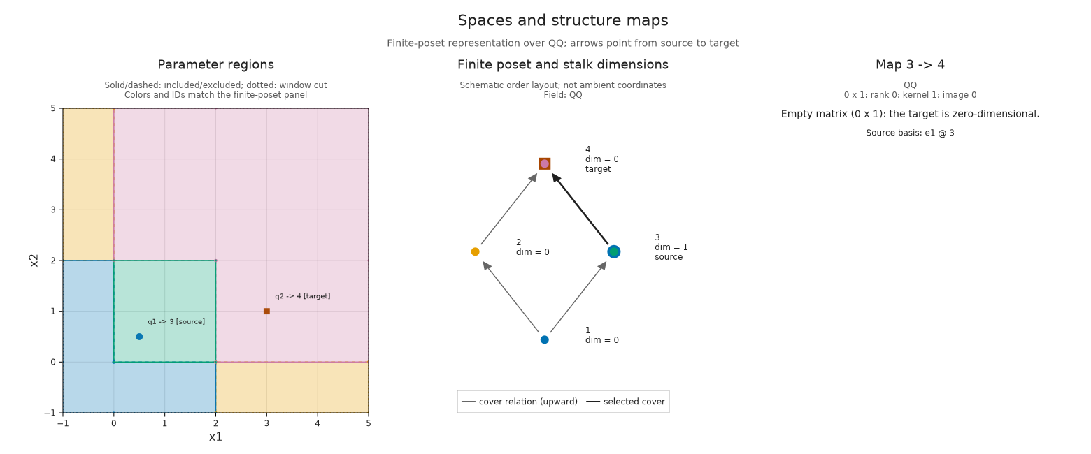
Now choose $u=(1/4,3/2)$ and $v=(3/2,1/4)$. Both lie inside the square. One coordinate increases while the other decreases, so neither point is at most the other. Predict whether sharing a finite label supplies a map between these original parameters.
To inspect the answer as data as well as a picture, visual_spec prepares the view without drawing it. visual_metadata retains its mathematical readout. We can render that same specification afterward.
u, v = (1//4, 3//2), (3//2, 1//4)
@assert OA.locate(classifier, u) == OA.locate(classifier, v) == inside_id
unordered_spec = OA.visual_spec(enc; kind=:module_inspector,
    parameter_pair=(u, v), box=view_box)
unordered = OA.visual_metadata(unordered_spec).inspection
@assert !unordered.defined && unordered.matrix === nothing
(; relation=unordered.relation, map_defined=unordered.defined)
(relation = :incomparable, map_defined = false)OP.visualize(unordered_spec)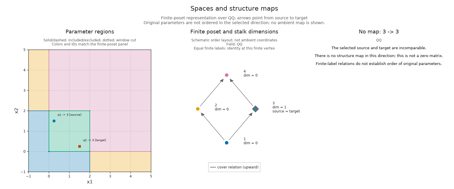
The shared finite label has an identity endomorphism, but the original module only prescribes maps for comparable parameters. Asking about the finite pair (inside_id, inside_id) would be a different question.
| Query in the original plane | What the encoding recovers |
|---|---|
| $x\leq y$, both inside | An identity map of rank one |
| $x\leq z$, leaving the square | A defined zero map of size $0\times1$ |
| $u$ and $v$, incomparable | No structure map to recover |
Outside the square is still inside this module's parameter domain. The zero-dimensional stalk at $z$ is represented by a real finite label. It is different from classifier sentinel 0, which some other encodings use for an unrepresented parameter.
Change the example: two overlapping squares
Add $[1,3]^2$ as an independent summand, keeping the first square $[0,2]^2$. The $2\times2$ identity coefficient matrix says that the two square contributions are independent. Along the increasing path
\[a=(1/2,1/2)\leq b=(3/2,3/2)\leq c=(5/2,5/2),\]
the first square alone is present at $a$, both are present at $b$, and only the second remains at $c$. Predict the three dimensions. Then predict whether any vector from $a$ survives all the way to $c$.
two_squares = OP.encode(
    [OA.BoxUpset([0, 0]), OA.BoxUpset([1, 1])],
    [OA.BoxDownset([2, 2]), OA.BoxDownset([3, 3])],
    OP.QQ[1 0; 0 1], options);
Follow the same recovery procedure: locate each original parameter and read the dimension at its finite label. The original enc remains available for comparison.
a, b, c = (1//2, 1//2), (3//2, 3//2), (5//2, 5//2)
two_classifier = OP.encoding_map(two_squares)
two_dims = OP.dimensions(two_squares)
qa, qb, qc = [OA.locate(two_classifier, p) for p in (a, b, c)]
path_dims = two_dims[[qa, qb, qc]]
@assert path_dims == [1, 2, 1]
path_dims
3-element Vector{Int64}:
1
2
1The dimensions are $1\to2\to1$. In coordinates that name the two summands, the maps are
\[\mathbb Q\ \xrightarrow{\;\left[\begin{smallmatrix}1\\0\end{smallmatrix}\right]\;} \mathbb Q^2\ \xrightarrow{\;\left[\begin{smallmatrix}0&1\end{smallmatrix}\right]\;}\ \mathbb Q.\]
The first map puts a vector into the first coordinate. The second discards that coordinate and keeps the second. Their composite is zero. The package may choose other bases; its stored matrices still compose because every query uses the same finite module.
two_module = OP.encoding_module(two_squares)
first_map = OA.structure_map(two_module; source=qa, target=qb)
second_map = OA.structure_map(two_module; source=qb, target=qc)
direct_map = OA.structure_map(two_module; source=qa, target=qc)
@assert size(first_map) == (2, 1) && size(second_map) == (1, 2)
@assert first_map != zeros(OP.QQ, 2, 1) && second_map != zeros(OP.QQ, 1, 2)
@assert second_map * first_map == direct_map == zeros(OP.QQ, 1, 1)
(; first_map, second_map, composite=direct_map)
(first_map = Rational{BigInt}[1; 0;;], second_map = Rational{BigInt}[0 1], composite = Rational{BigInt}[0;;])Read the first step in the inspector. The source has one coordinate and the overlap has two, so the matrix is a column. We retain the same viewing window; it contains both squares.
OP.visualize(two_squares; kind=:module_inspector,
    parameter_pair=(a, b), box=view_box)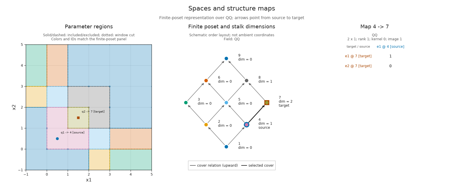
Next leave the overlap for the second square. The matrix is a row, and its rank is again one. The surviving coordinate belongs to the second summand, not the first.
OP.visualize(two_squares; kind=:module_inspector,
    parameter_pair=(b, c), box=view_box)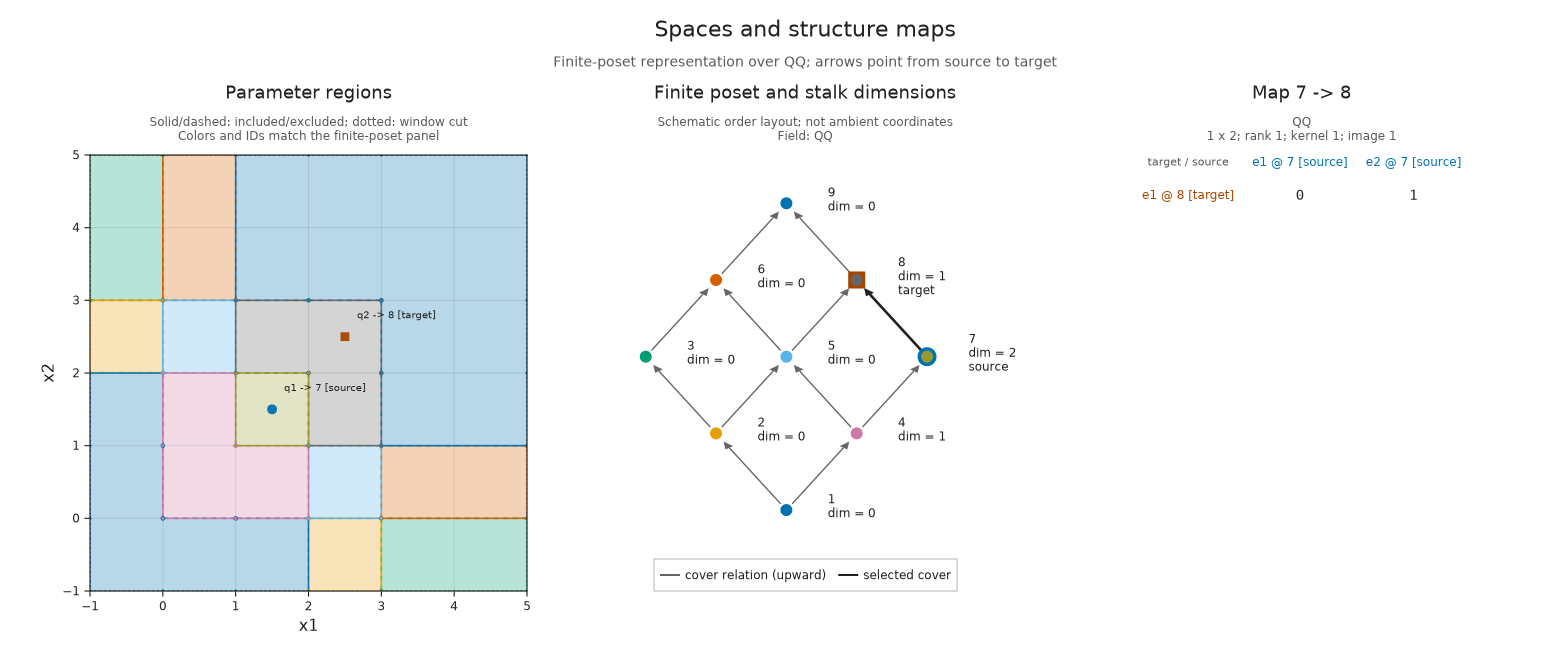
Finally select the endpoints. This time both stalks have dimension one, yet the matrix is $[0]$. Unlike the earlier $0\times1$ map, it has a row and a column: the target space exists, but nothing from the source reaches it.
OP.visualize(two_squares; kind=:module_inspector,
    parameter_pair=(a, c), box=view_box)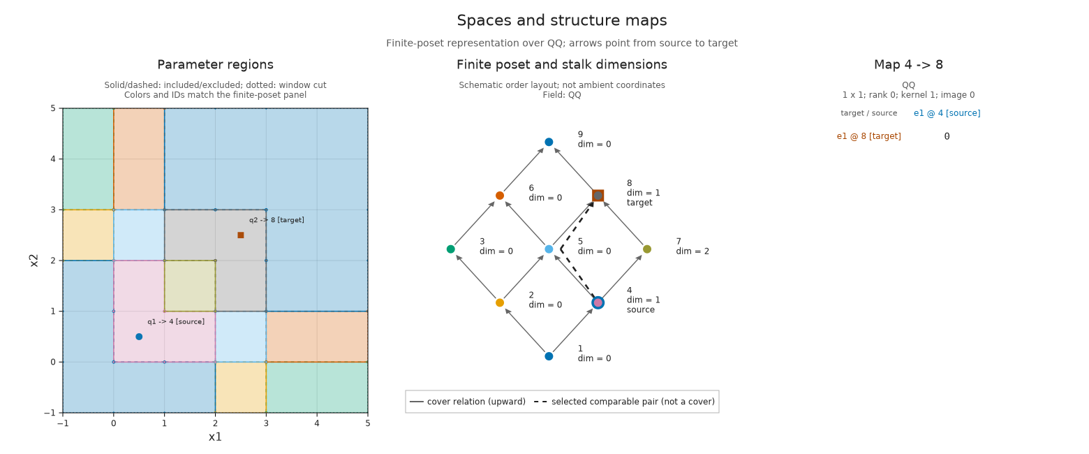
The nonzero vector at the beginning and the nonzero vector at the end belong to different summands. Dimensions $1,2,1$ alone cannot tell us this. Even the two adjacent ranks, both one, do not determine the rank of the composite. The actual maps supply the missing information.
We have now answered the opening question: a finite encoding recovers a space by locating its parameter, and a structure map by locating a comparable pair. The static figures retain those choices and their answers. The following sections explore how the presentation creates the spaces, how to change selections interactively, and how to export a figure. Each can be skipped.
Optional: Where the spaces and maps come from
The two-square input also explains the spaces as images of small matrices. At a parameter, keep the rows whose downsets contain it and the columns whose upsets contain it. The resulting active block maps active source coordinates to active target coordinates. Its image is the stalk. For our identity coefficient matrix, predict these blocks:
| Parameter | Active rows | Active columns | Block | Image dimension |
|---|---|---|---|---|
| $a$ | $D_1,D_2$ | $U_1$ | $[1\;0]^T$ | 1 |
| $b$ | $D_1,D_2$ | $U_1,U_2$ | $I_2$ | 2 |
| $c$ | $D_2$ | $U_1,U_2$ | $[0\;1]$ | 1 |
encoding_presentation retrieves the finite fringe presentation retained by this encoding. presentation_stalk inspects one of its stalks. These queries use the retained presentation's coordinates; they do not assume those coordinates match every stored module basis.
retained_fringe = OP.encoding_presentation(two_squares)
@assert retained_fringe !== nothing
overlap = OA.presentation_stalk(two_squares; vertex=qb)
@assert OA.active_rows(overlap) == [1, 2]
@assert OA.active_columns(overlap) == [1, 2]
@assert OA.presentation_matrix(overlap) == OP.QQ[1 0; 0 1]
OA.presentation_matrix(overlap)
2×2 Matrix{Rational{BigInt}}:
1 0
0 1The active block is the identity, so its image is the entire two-dimensional target. Request basis=true to retain vectors spanning that image. Each column of image_basis is an actual vector in the active downset coordinates. Without this option, a single-stalk query returns the block and its rank without computing an image basis.
overlap_with_basis = OA.presentation_stalk(two_squares; vertex=qb, basis=true)
@assert OA.image_basis(overlap_with_basis) == OP.QQ[1 0; 0 1]
OA.image_basis(overlap_with_basis)
2×2 Matrix{Rational{BigInt}}:
1 0
0 1Try $t=(1/2,5/2)$. It lies in $U_1$ and $D_2$, but in neither $U_2$ nor $D_1$. The active block keeps row 2 and column 1 of the identity matrix: it is $[0]$. What shape must an embedded basis of its image have?
t = (1//2, 5//2)
qt = OA.locate(two_classifier, t)
zero_stalk = OA.presentation_stalk(two_squares; vertex=qt, basis=true)
@assert OA.active_rows(zero_stalk) == [2]
@assert OA.active_columns(zero_stalk) == [1]
@assert OA.presentation_matrix(zero_stalk) == reshape(OP.QQ[0], 1, 1)
@assert size(OA.image_basis(zero_stalk)) == (1, 0)
(; block=OA.presentation_matrix(zero_stalk),
   image_basis_size=size(OA.image_basis(zero_stalk)))
(block = Rational{BigInt}[0;;], image_basis_size = (1, 0))The basis has one row and zero columns: it embeds the zero space in a one-dimensional ambient target. Having an active source and an active target does not force their coefficient to be nonzero.
The presentation inspector shows the two supports, the full coefficients, the active block, and its image basis. upset=1 and downset=2 choose the supports to draw; they do not change the active-block calculation. basis=true asks to show its image basis as well.
OP.visualize(two_squares; kind=:presentation_inspector,
    point=t, upset=1, downset=2, basis=true, box=view_box)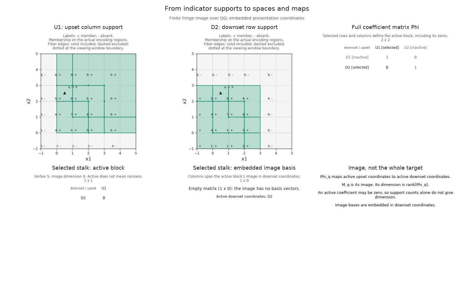
To recover a map, let $B_b$ and $B_c$ denote the image-basis matrices at its source and target. The ambient projection $R$ drops downset coordinates that have disappeared. The induced map $C$ between image coordinates satisfies
\[B_c C=R B_b.\]
The right side first embeds a source vector and then projects it. On the left, $C$ gives the target image coordinates and $B_c$ embeds them into the active target coordinates. For the step $b\leq c$ in our path, the ambient projection keeps only the second coordinate. presentation_map computes the endpoint bases needed to express this map.
presentation_bc = OA.presentation_map(two_squares; source=qb, target=qc)
Bb = OA.image_basis(OA.source_stalk(presentation_bc))
Bc = OA.image_basis(OA.target_stalk(presentation_bc))
R = OA.ambient_projection(presentation_bc)
C = OA.induced_map(presentation_bc)
@assert R == OP.QQ[0 1]
@assert Bc * C == R * Bb
C
1×2 Matrix{Rational{BigInt}}:
0 1The figure places the active blocks, bases, projection, and induced map together. Compare them with the equation. This diagonal example gives the familiar row $[0\;1]$; for a general presentation, matching a nonzero matrix to the separately stored module may require a change of basis. The indicator-presentation chapter explains why these image spaces and maps fit together.
OP.visualize(two_squares; kind=:presentation_inspector,
    parameter_pair=(b, c), upset=1, downset=2, box=view_box)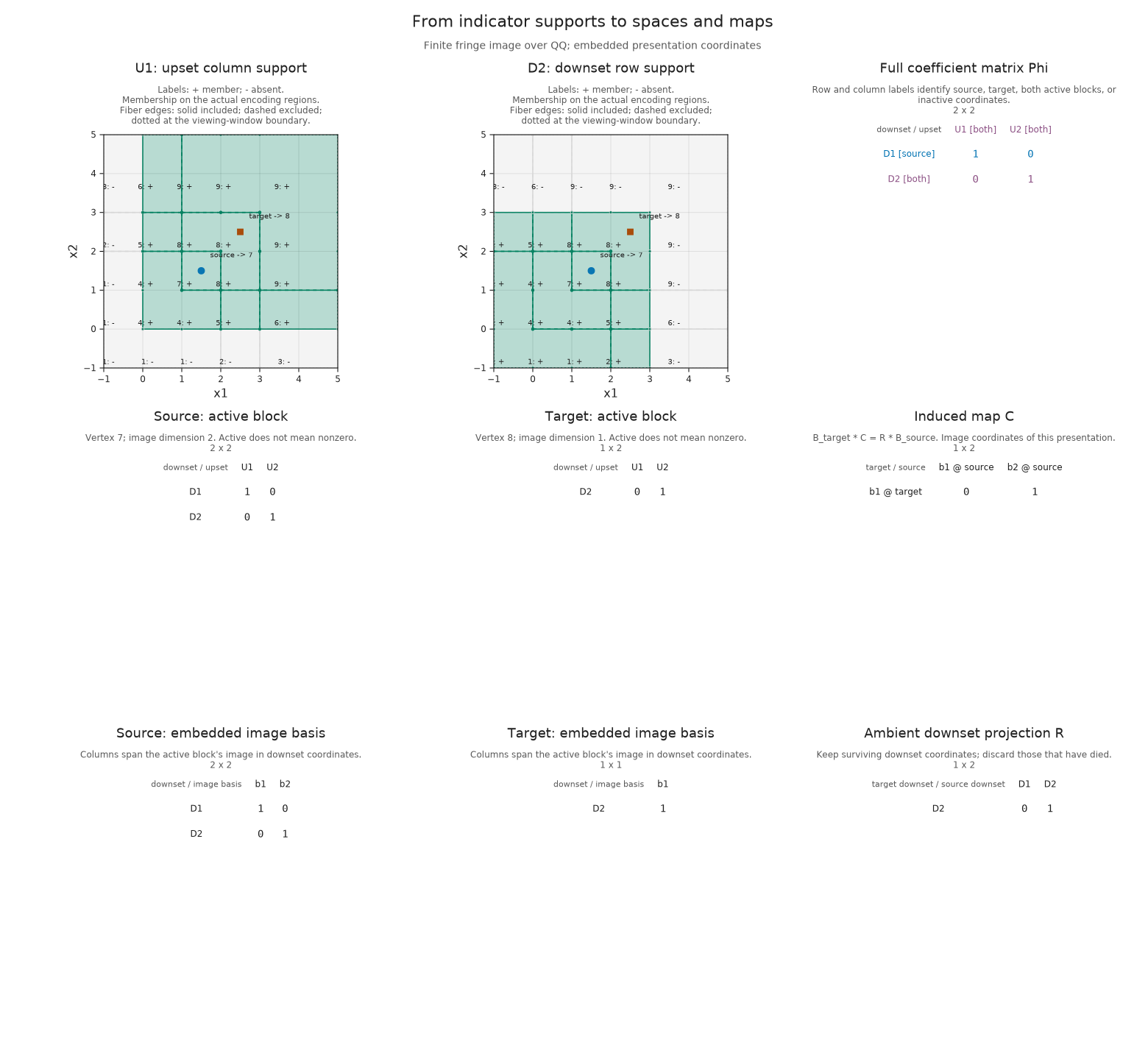
Optional: Explore a live linked view
The saved figures answer the lesson's questions without a server. To change the selection in a browser, install WGLMakie in your notebook environment and keep the Julia kernel running. The optional integrations guide explains the plotting packages. Run these Julia commands in a new notebook cell when you want a live view; they are not part of the static publication run.
import WGLMakie
live = OP.inspection_session(two_squares; box=view_box)
OA.select_inspection!(live; parameter_pair=(a, c))
OP.visualize(live; backend=:wglmakie)
Start with the endpoint map: the matrix should be $[0]$. Select a stalk in Selection endpoint, then use the exact point fields to inspect (3/2, 3/2) in the overlap. Its dimension is two. To return to the original pair, enter source (1/2, 1/2) and target (5/2, 5/2) in the exact parameter-pair fields. Fractions such as 1/2 are accepted as exact input; pointer clicks use drawing coordinates and are less useful for boundary questions.
If you read the presentation section, switch Coordinate view to presentation and inspect (1/2, 5/2) with Compute selected image basis enabled. The active block is $[0]$ and its basis has shape $1\times0$. Switching views preserves the selection, but does not identify the two coordinate bases.
A snapshot keeps the selected state as a static specification:
snapshot = OA.inspection_snapshot(live)
OP.visualize(snapshot; backend=:cairomakie)
Each visualize(live; backend=:wglmakie) call creates a new viewer linked to the same session; display a given viewer in one browser client. Closing a browser viewer leaves the session available. When finished, use Close inspector or run OA.close_inspection!(live). The snapshot remains usable afterward.
Optional: Save a figure
The notebook already retains its static results. To save a separate PNG or SVG, use save_visual with the same mathematical selection. We will export the two-square endpoint map, whose zero entry answers the variation's question.
The files go under tamerop_outputs/square in your working directory. export_path returns each actual path. The recipe supplies the figure layout; no styling changes are required.
output_dir = joinpath("tamerop_outputs", "square")
png = OP.save_visual(output_dir, "two-square-composite", two_squares;
    kind=:module_inspector, parameter_pair=(a, c), box=view_box,
    format=:png, backend=:cairomakie)
@assert isfile(OP.export_path(png))
OP.export_path(png)"tamerop_outputs/square/two-square-composite.png"SVG preserves sharp lines and text when resized. Keep the same selection and change the format. Stating the static backend here also works if you have loaded WGLMakie for the optional live view.
svg = OP.save_visual(output_dir, "two-square-composite", two_squares;
    kind=:module_inspector, parameter_pair=(a, c), box=view_box,
    format=:svg, backend=:cairomakie)
@assert isfile(OP.export_path(svg))
OP.export_path(svg)"tamerop_outputs/square/two-square-composite.svg"When can we do this beyond the square?
A finite label is useful because it comes with both a space and the maps needed to recover the original module. Our square used four labels, including a disconnected fiber. The two-square variation showed why the maps matter: two rank-one steps can have zero composite.
These constructions give us finite descriptions for the particular presentations we supplied. The next question is when a persistence module admits such a description at all. Continue with tameness and scope to relate constant subdivisions, finite encodings, and finite presentations. For other views of the objects just inspected, consult the visualization guide.