Ordinary persistence: TamerOp and PHAT
Study completed 2026-10-04. Both programs returned verified complete barcodes for all 48 fixed inputs. TamerOp was 1.33× as fast in the balanced aggregate for native construction plus the complete query, corresponding to about 25% less time (approximate 95% ratio interval 1.290–1.370×). Graphs show the strongest family advantage; the algebraic controls have similar aggregate performance, with PHAT slightly faster.
These are compiled computations with previous mathematical results discarded. Inputs range from 387 to 1,048,576 cells. The largest complete 3-skeleton takes about 3.86 s in TamerOp and 7.14 s in PHAT. Individual results vary, and several favor PHAT. The supported conclusion is an aggregate and family-specific advantage; the study's predeclared criteria for “generally faster on this suite” were not met.
All benchmark results · Runtimes and sizes · Scaling curves · Machine and versions · Download the results
Why compare ordinary persistence?
As a filtration grows, components, holes and higher-dimensional classes appear and disappear. Their lifetimes form the ordinary barcode. This is a natural complete-result comparison: both programs receive the same filtered boundary matrix and must recover the same intervals in every supplied degree.
The inputs specify cell dimensions, integer filtration grades and boundary columns over F₂. The answer contains every nonempty finite interval and every essential birth. Equal-grade, zero-length pairs are omitted; surviving classes are neither discarded nor clipped. For this finite one-parameter problem, the complete barcode determines the persistence module up to isomorphism.
TamerOp answers directly from a GradedComplex through public persistence_diagram(...; representatives=false). This route does not construct an EncodingResult. Finite encodings remain central when later questions need the retained module and maps, especially with several parameters; see ordinary persistence and finite encodings.
The comparison uses unchanged upstream PHAT v1.7 with its default twist reduction and bit-tree pivot columns, on one thread. It concerns that supported default route, rather than a survey of all PHAT algorithms or threaded configurations.
What was measured?
Native construction converts shared decoded boundary data into each program's representation. The query reduces it and materializes a sorted complete barcode. PHAT's conversion from cell pairs and recovery of essential births are charged. TamerOp's ordinary public validation remains enabled. The primary measurement includes construction and the complete query in one timer.
| Phase | PHAT/TamerOp (95% interval) |
|---|---|
| Native construction | 0.508 (0.452–0.571) |
| Complete barcode query | 1.629 (1.573–1.686) |
| Construction plus query | 1.329 (1.290–1.370) |
All ratios divide PHAT time by TamerOp time; values above one favor TamerOp. The intervals use five paired process passes. The combined measurement is taken directly, not obtained by adding separately measured medians. PHAT spends less time on native construction, while TamerOp's lower query times produce the combined advantage on this suite.
Parsing, fixture generation, independent checks, reset inspection, answer serialization, package loading and compilation are outside the timers. Filtration construction from raw images or point clouds is also outside this supplied-boundary comparison.
Each phase uses two fresh warmups and three accepted measurements per process pass. Every request begins with an unreduced PHAT matrix or an input-only TamerOp complex, with no previous barcode or reduction reused. Reset checks reject corrupted native inputs. Both programs may reuse intermediate work within a request. Julia performs a full collection before phase warmup and charges natural collections during requests.
Five serial paired passes produced 4,320 accepted samples and 2,880 warmup rows. Every accepted measurement recorded zero compilation and recompilation; no contaminated attempts were rejected. Tool and case order reverse in alternating passes. Every produced barcode, including warmups, is checked outside the timer.
Results by input family
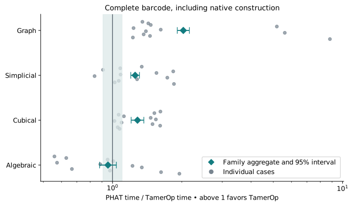
The ratios below use construction plus the complete query. Each family contains four structural variants at three measured sizes, with equal declared weight. The confidence intervals describe variation across the five paired passes.
| Family | Cases | PHAT/TamerOp (95% interval) | Practical interpretation |
|---|---|---|---|
| Graph | 12 | 2.031 (1.912–2.158) | TamerOp 2.03× as fast |
| Simplicial | 12 | 1.254 (1.201–1.310) | TamerOp 1.25× as fast |
| Cubical | 12 | 1.284 (1.205–1.368) | TamerOp 1.28× as fast |
| Algebraic | 12 | 0.955 (0.878–1.039) | Similar; PHAT about 4.5% less time |
The largest displayed case-median saving for TamerOp is about 3.28 seconds on the largest complete 3-skeleton. PHAT's largest saving is about 0.53 ms on the middle-sized joined-sphere input: 3.67 ms versus TamerOp's 4.19 ms. These differences describe the measured requests, not an estimated total for an unmeasured workload.
A similar family aggregate can conceal substantial individual differences. PHAT has a clear relative advantage on the low-density algebraic controls. The smallest takes about 0.049 ms in PHAT and 0.087 ms in TamerOp, with a paired ratio of 0.559. That absolute difference is small for one request but may matter across frequent batches.
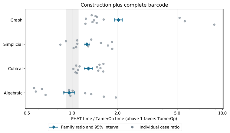
The blue diamonds summarize ratios, not standalone TamerOp runtimes. Gray points retain all twelve cases per family. The vertical line marks equal time; the pale band spans the declared practical range from 1/1.10 to 1.10. It indicates similar point estimates, not statistical equivalence. The spread of algebraic cases explains why its aggregate alone is insufficient. Open the full-size figure.
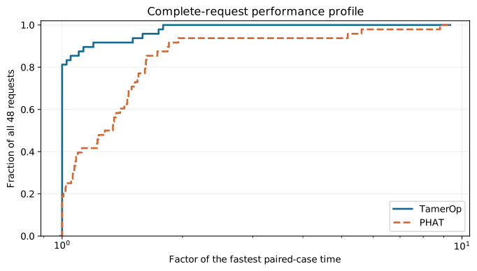
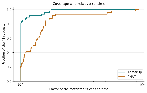
The horizontal axis allows a larger factor of the fastest paired-case time; the vertical axis is the fraction of all 48 requests within that factor. The profile uses the same paired geometric case ratios as the family comparison, with equal weight for each case. TamerOp reaches full coverage at a smaller factor, while both programs complete every request. This describes relative time and coverage; the tables below show the actual waiting times. Open the full-size figure.
Actual runtimes and input sizes
All times in this table and the scaling figures are milliseconds (1,000 ms = 1 second). Each time cell gives the median across the four structural variants at a family/size level, followed by the minimum and maximum in parentheses. Each case time is itself the median of five process medians. These ranges describe different inputs, not timing confidence intervals.
| Family / level | Cells | Boundary entries | Output bars | TamerOp ms | PHAT ms |
|---|---|---|---|---|---|
| Graph / 1 | 8,191–20,480 | 8,190–32,768 | 2,817–13,587 | 0.439 (0.418–1.303) | 0.632 (0.582–6.478) |
| Graph / 2 | 32,767–81,920 | 32,766–131,072 | 11,427–54,064 | 2.092 (1.933–6.324) | 2.900 (2.706–38.809) |
| Graph / 3 | 131,071–327,680 | 131,070–524,288 | 45,622–216,621 | 9.381 (8.983–26.870) | 13.217 (13.009–246.669) |
| Simplicial / 1 | 5,488–24,157 | 11,656–92,484 | 1,202–17,852 | 1.140 (0.392–39.957) | 1.392 (0.449–72.679) |
| Simplicial / 2 | 43,744–102,090 | 98,304–396,760 | 11,683–82,973 | 14.929 (4.193–452.904) | 20.629 (3.667–779.382) |
| Simplicial / 3 | 212,993–396,606 | 393,216–1,555,400 | 46,708–342,462 | 144.954 (17.930–3,862.012) | 190.942 (17.990–7,141.729) |
| Cubical / 1 | 12,167–16,384 | 32,004–41,472 | 447–1,098 | 1.143 (1.004–1.569) | 1.577 (1.281–1.715) |
| Cubical / 2 | 59,319–262,144 | 173,394–524,288 | 2,147–17,439 | 14.284 (7.062–21.993) | 20.309 (7.399–33.311) |
| Cubical / 3 | 250,047–1,048,576 | 738,234–2,097,152 | 8,915–69,567 | 70.654 (34.985–101.147) | 95.072 (38.608–153.654) |
| Algebraic / 1 | 387–396 | 2,218–9,068 | 137–163 | 0.140 (0.087–0.164) | 0.122 (0.049–0.171) |
| Algebraic / 2 | 771–780 | 4,729–38,762 | 294–314 | 0.415 (0.206–0.586) | 0.463 (0.120–0.796) |
| Algebraic / 3 | 1,539–1,548 | 11,470–157,959 | 575–607 | 1.307 (0.492–2.199) | 1.948 (0.330–4.679) |
Cells count generators in all supplied degrees; boundary entries count nonzero coefficients. Output bars include finite intervals and essential births. Algebraic controls have fewer cells but much denser boundaries. A size level is a position within a variant's ladder, not a shared geometric scale.
For a direct comparison of the endpoints, these are the largest inputs of all sixteen variants:
| Family / variant | Cells | Boundary entries | TamerOp ms | PHAT ms | PHAT/TamerOp |
|---|---|---|---|---|---|
| Graph / Path forest | 131,071 | 131,070 | 9.197 | 13.009 | 1.366 |
| Graph / Single cycle | 131,072 | 131,072 | 8.983 | 13.212 | 1.455 |
| Graph / Disconnected cycles | 131,072 | 131,072 | 9.564 | 13.223 | 1.226 |
| Graph / Graph with extra edges | 327,680 | 524,288 | 26.870 | 246.669 | 8.814 |
| Simplicial / Complete 2-skeleton | 349,632 | 1,040,384 | 246.686 | 336.172 | 1.279 |
| Simplicial / Triangulated disk | 391,171 | 781,320 | 43.221 | 45.712 | 1.064 |
| Simplicial / Joined sphere boundaries | 212,993 | 393,216 | 17.930 | 17.990 | 1.022 |
| Simplicial / Complete 3-skeleton | 396,606 | 1,555,400 | 3,862.012 | 7,141.729 | 1.850 |
| Cubical / Open 2D grid | 1,046,529 | 2,091,012 | 101.147 | 145.291 | 1.492 |
| Cubical / Periodic 2D grid | 1,048,576 | 2,097,152 | 99.329 | 153.654 | 1.611 |
| Cubical / Open 3D grid | 250,047 | 738,234 | 34.985 | 38.608 | 1.053 |
| Cubical / Periodic 3D grid | 262,144 | 786,432 | 41.979 | 44.854 | 1.074 |
| Algebraic / 2 transvections/cell | 1,539 | 11,470 | 0.492 | 0.330 | 0.666 |
| Algebraic / 4 transvections/cell | 1,542 | 47,878 | 0.909 | 0.951 | 0.974 |
| Algebraic / 8 transvections/cell | 1,545 | 119,270 | 1.706 | 2.946 | 1.625 |
| Algebraic / 16 transvections/cell | 1,548 | 157,959 | 2.199 | 4.679 | 1.953 |
Dividing the displayed medians can differ from the reported ratio: ratios pair process passes before aggregation, whereas these times summarize each tool separately. The complete CSV retains every size and all three timing phases.
How runtime changes with input size
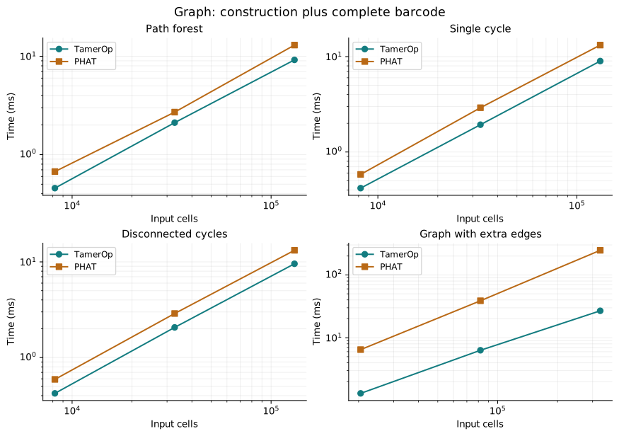
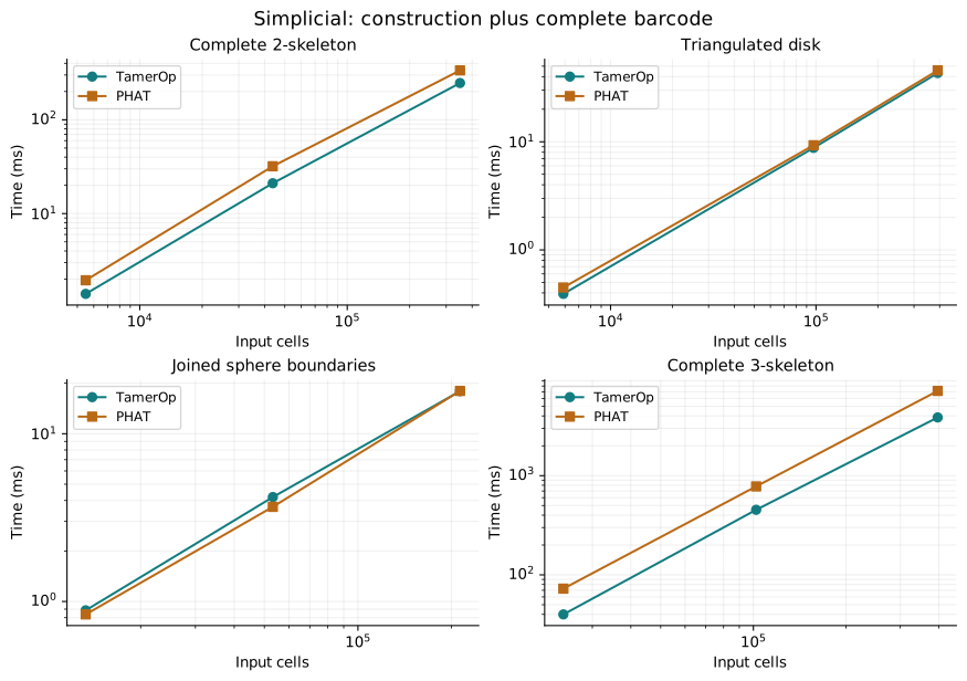
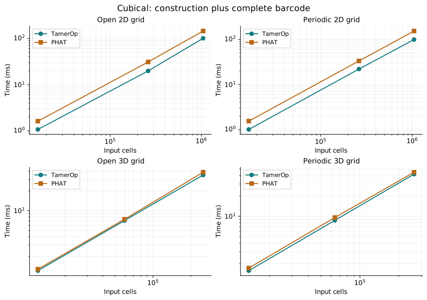
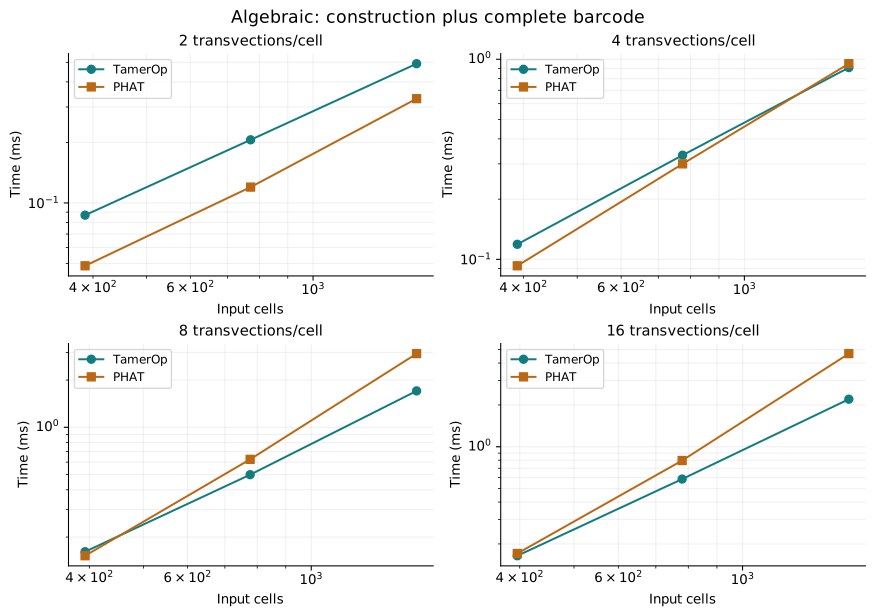
Each panel follows one structural variant through its three measured sizes. TamerOp is the solid blue line with circles; PHAT is the dashed orange line with squares. Both axes are logarithmic, and panel limits vary to keep each sequence legible. The lines guide the eye between observations; they are not asymptotic predictions. All panels include native construction and the complete barcode query. The per-case data provide the exact values.
Graphs
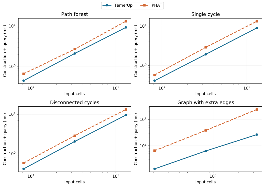
Every graph case favors TamerOp beyond the practical band. The largest relative separation occurs for graphs with extra edges: at the largest size, the programs take about 26.87 ms and 246.67 ms, respectively. The simpler graph variants have smaller but consistent advantages. Open the full-size figure.
Simplicial inputs
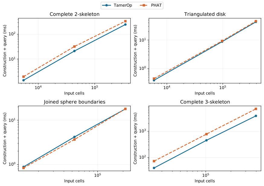
The complete 3-skeleton accounts for the largest absolute saving in the suite. The largest disk and joined-sphere inputs have similar runtimes instead, and the middle-sized joined-sphere input favors PHAT. These differences would be lost in a single curve joining all simplicial inputs. Open the full-size figure.
Cubical grids
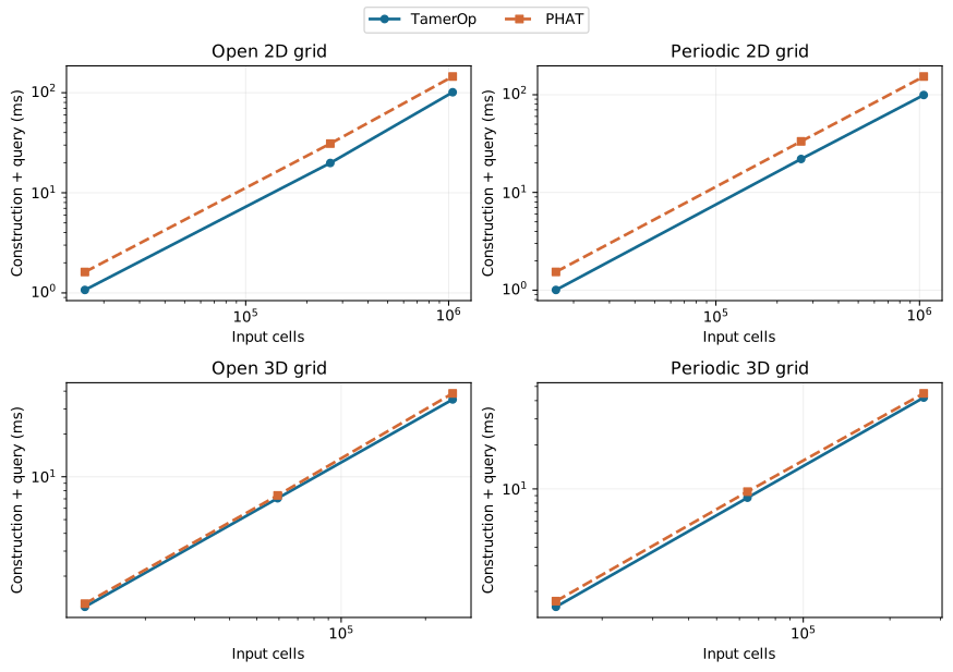
The two-dimensional grids show a larger separation than the three-dimensional grids. At the largest sizes, TamerOp uses about 99–101 ms for the two-dimensional grids and PHAT about 145–154 ms. The largest three-dimensional cases fall within the practical band, with TamerOp's measured times slightly lower. Open the full-size figure.
Algebraic controls
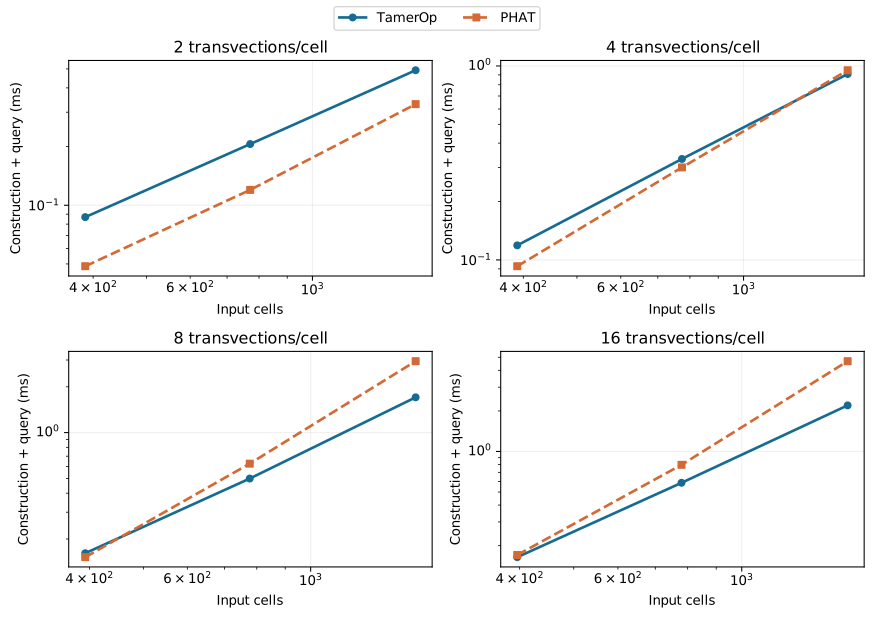
These controls change the density of the boundary matrices while retaining a known barcode. PHAT is faster on all three lowest-density inputs. With eight or sixteen transvections per cell, the larger inputs favor TamerOp instead. Cell count alone does not explain the computational difficulty. Open the full-size figure.
How were answers and aggregates checked?
The examples are synthetic and cover four families with different topology and boundary structure. Algebraic controls apply compatible filtered basis changes to elementary intervals, changing arithmetic difficulty while retaining a known barcode. The independent evidence varies by family:
| Inputs | Independent evidence in addition to complete cross-tool agreement |
|---|---|
| All 48 cases | Exact filtration, dimensions and d² = 0 checks. |
| 12 graph cases | Complete barcode derived from DFS component-map ranks and graph cycle counts. |
| 12 algebraic cases | Known complete barcode preserved by compatible filtered changes of basis. |
| 12 simplicial and 12 cubical cases | Known terminal Betti numbers. This does not independently certify every birth and death. |
| Eight unscored small controls | Complete rank-invariant oracle and hand-derived answers. |
All 56 qualification inputs matched in TamerOp and PHAT's twist and standard reductions; only twist is timed. Fifteen harness checks passed, covering malformed inputs, incorrect or incomplete answers, cache resets, compilation rejection and fixed-suite selection. Source-identical library acceptance checks were credited; the package-wide suite was not rerun for this comparison.
Each family receives one quarter of the total weight, divided equally among its four variants and three sizes. Within a pass, each tool's median of three samples gives its time. Case ratios are geometric means of the five paired PHAT/TamerOp process-median ratios. Family and overall aggregates use those fixed weights. The approximate 95% intervals are t intervals on five paired-block log aggregates, with four degrees of freedom. They describe repeat-run variation on these fixed inputs and this host, not uncertainty over arbitrary future data.
For the combined measurement, the aggregate is 1.329 with interval 1.290–1.370 and a pass range of 1.277–1.363. Equal-case weighting gives the same result because the families and variants contain equal numbers of cases. The supplementary classification counts use the predeclared practical band:
| Family | TamerOp faster | Within the practical band | PHAT faster |
|---|---|---|---|
| Graph | 12 | 0 | 0 |
| Simplicial | 6 | 4 | 2 |
| Cubical | 7 | 5 | 0 |
| Algebraic | 4 | 3 | 5 |
The counts support the interpretation of the ratios; a saving of several seconds and a microsecond difference do not have equal practical importance. The broad claim gate requires at least 80% weighted practical advantages, 80% of families favoring TamerOp, and an aggregate lower interval above 1.10, supported by pass ranges and equal-case sensitivity. Here the first two shares are 60.4% and 75%. The predeclared criteria for “generally faster on this suite” are not met. The supported conclusion is the aggregate and family-specific comparison above.
The sixteen largest inputs underwent a bounded feasibility pilot. Every proposed endpoint fit the budget and was retained. No implementation tuning, favorable case selection or weight changes followed those measurements. Source, fixtures, adapters, protocol and runtime identities were frozen before confirmation. There is no separate held-out performance claim. No pilot or earlier-study timings enter the reported score.
Machine and versions
These specifications describe the actual measured candidate and run.
| Component | Recorded configuration |
|---|---|
| CPU | 13th Gen Intel(R) Core(TM) i7-1365U |
| Logical CPUs / usable RAM | 12 / 31.00 GiB reported by Linux |
| OS | x86-64 Linux 6.8.0-106-generic |
| Julia | 1.12.1 |
| TamerOp source | Accepted development snapshot phat-2026-10-04; comparison candidate phat-v2-2026-10-04 |
| PHAT | v1.7, commit a74705e4628e447084d47dbf13a16dfb6d2ebd9a |
| C++ build | g++ (Ubuntu 11.4.0-1ubuntu1~22.04.3) 11.4.0; -O3 -DNDEBUG -std=c++17 |
| Parallelism | One computation thread; serial workers; one Julia/BLAS thread |
This was a shared desktop with five-second resource monitoring. During final confirmation, one-minute load ranged from 1.42 to 2.33 and available memory stayed above 7.39 GiB. System pressure and swap observations are retained in the metadata; they cannot be attributed to either tool alone.
Limits were 60 seconds per operation, 900 seconds per worker and 4 GiB sampled worker RSS, with 20 minutes for the pilot and 100 for confirmation. The operation watchdog includes untimed setup and checks, so it is not an exact query-time cutoff. No worker failed or reached a resource limit. Fixture generation, qualification, the pilot and confirmation took about 2.0, 1.1, 6.1 and 19.1 minutes, respectively; preparation and report building are outside the timing allowance.
The source snapshot includes changes beyond its Git base and is not a tagged release. The provenance record identifies the exact source, adapters, runtime and inputs. PHAT v2 uses a different workload distribution from the earlier small-input comparison, with the same accepted implementation snapshot. A changed aggregate across those studies is not itself an implementation speedup.
Memory
TamerOp used substantially more process memory despite its lower aggregate computation time:
| Tool | Sampled peak worker RSS (MiB) |
|---|---|
| TamerOp | 1,392.1–1,540.5 |
| PHAT | 155.8–155.8 |
These are ranges of sampled peak worker RSS, including the runtime, compiled code, temporary storage and untimed work. They are not retained mathematical storage, and brief peaks may be missed. Julia supplies separate per-request measurements:
| Julia measurement | Range across complete requests (MiB) |
|---|---|
| Allocation traffic during the request | 0.109–176.912 |
| Retained native input | 0.043–54.001 |
| Retained normalized barcode | 0.003–8.131 |
Allocation traffic counts bytes allocated during the call, not simultaneous memory usage. Retained input and barcode sizes are separate Base.summarysize roots. PHAT's allocation and retained-object counters are unavailable and remain null rather than zero. The speed comparison and these memory measurements answer different questions.
Data and reproducibility
The public results accompany this page:
- Summary JSON: aggregates, completion, memory and host observations.
- Per-case CSV: all 144 case/phase summaries, with exact sizes, times and ratios.
- Per-pass observations: times, allocations and retained sizes.
- Provenance and machine metadata and original download checksums.
- Data dictionary: units, row meanings, uncertainty and missing values.
- Figure presentation record and figure checksums: the QPA-style exports used here.
- Original sealed figures: ratios, profile, graphs, simplicial inputs, cubical grids, and algebraic controls.
The figures are rendered from the unchanged PHAT v2 summaries using the shared benchmark style. The figure renderer can regenerate them with Python and Matplotlib, without running benchmarks. Its presentation record identifies the input summaries, style and renderer; the original sealed files remain available alongside the new exports.
The downloads support inspection and recomputation of the summaries. Exact inputs, validators, raw rows, source snapshots and commands remain in the local evidence archive; this is not yet an executable reproduction bundle or an independent clean-machine replication.
The study covers complete ordinary F₂ barcodes from supplied boundaries. It does not compare raw-data ingestion, representative cycles, other fields, cohomology, relative or extended persistence, zigzags, incremental updates, multiparameter computations, startup or every PHAT setting. For measuring your own workload, follow the benchmarking manual.