Persistence modules over posets
When a shape changes with a parameter, we can ask how many connected components or holes it has. We can also ask a more revealing question: how does a class observed at one parameter continue to another? A persistence module records the vector spaces in which these classes live and the linear maps that follow them through the changes.
This page develops that idea from the ring lesson. We will see why several parameters lead to a partially ordered set, what a module over that set contains, and why keeping only the dimensions loses information. These are the ingredients needed to understand the next step: a finite encoding.
You need familiarity with vectors, linear maps, and matrix multiplication. No Julia installation or previous knowledge of homology is needed to follow the examples.
If you have just finished the ring notebook, why two parameters change the problem offers a shorter route to the square example. This chapter provides the fuller development, including the module axioms and why compositions must agree.
Begin with a ring that fills in
Imagine nine unit squares arranged in a three-by-three grid. Assign each square an appearance value:
\[\begin{pmatrix} 0 & 0 & 0 \\ 0 & 5 & 0 \\ 0 & 0 & 0 \end{pmatrix}.\]
At a real parameter $t$, include every square whose value is at most $t$, together with its edges and vertices. There are no identifications between opposite sides of the grid. Write $X_t$ for the resulting shape. Before 0 it is empty; from 0 up to 5 it is a ring; at 5 the center appears and fills the hole.
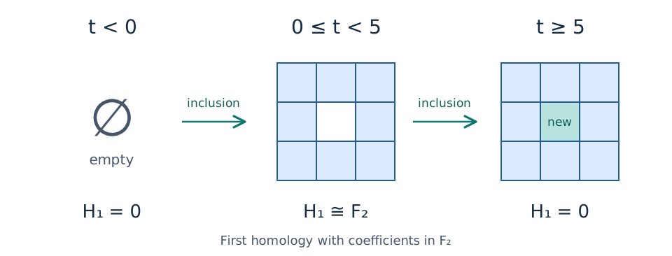
The squares enter at their assigned values. The arrows between shapes are inclusions. This is an authored schematic of the example; the vector spaces underneath describe its first homology over F₂.
Because squares are added and never removed, $X_s$ is contained in $X_t$ whenever $s\leq t$. Such a nested family is called a filtration. This is a sublevel filtration: membership is determined by a value being less than or equal to the parameter.
To describe its holes algebraically, fix the coefficient field $\mathbb{k}=\mathbb{F}_2$, the field with two elements. A field supplies the scalars for our vector spaces; in $\mathbb{F}_2$, addition is modulo two. The first homology space, written $H_1(X_t;\mathbb{k})$, records loops up to the relation that a loop bounding a filled patch represents zero. More generally, it allows linear combinations of loops with coefficients in $\mathbb{k}$.
For the ring, there is one independent nonzero loop class around the hole. Once the center is filled, that loop bounds a filled patch and its class is zero. Thus, if we write $M(t)=H_1(X_t;\mathbb{k})$, we obtain
\[M(t)\cong \begin{cases} \mathbb{k}, & 0\leq t<5,\\ 0, & t<0\text{ or }t\geq5. \end{cases}\]
Here $0$ denotes the zero vector space, which has only the zero vector. The subscript 1 in $H_1$ specifies the homological degree: we are studying loop classes. The dimension of $H_1$ tells us how many independent such classes there are. A degree-one homology space can have dimension zero, one, or more; the degree and the dimension are different quantities.
Follow the class through linear maps
The inclusion $X_s\subseteq X_t$ sends a loop in the earlier shape to the same loop in the later shape. It induces a linear map
\[M(s\leq t):M(s)\longrightarrow M(t).\]
The notation records both the starting parameter $s$ and the ending parameter $t$. This map tells us what becomes of every class from the earlier space. It is called a structure map of the persistence module.
For example, choose the loop around the ring as a basis for its one-dimensional homology. At parameters 1 and 4 the same loop generates the same class, so the map is represented by the identity matrix $[1]$. At parameter 5 that class becomes zero:
\[\underbrace{M(1)}_{\mathbb{k}} \xrightarrow{[1]} \underbrace{M(4)}_{\mathbb{k}} \xrightarrow{0} \underbrace{M(5)}_{0}.\]
The final arrow is the unique linear map from a one-dimensional space to the zero space. Its matrix has zero rows and one column; the label $0$ denotes that zero map. The direct map from parameter 1 to parameter 5 is also zero: following the class in two steps gives the same answer as following it in one step.
This example explains why an inclusion of shapes can induce a homology map that is not injective. The loop remains present as a geometric curve inside the filled square, but its homology class has become zero.
The barcode interval $[0,5)$ packages the life of this class. It includes 0 because the ring is already present there, and excludes 5 because the hole is already filled there. An interval module places one copy of the field at each parameter in its interval, zero elsewhere, and identity maps between parameters inside the interval. It therefore specifies maps as well as dimensions.
For a one-parameter filtration of a finite simplicial or cubical complex, homology over a field has a barcode that describes the resulting persistence module up to compatible changes of basis: the module is a direct sum of interval modules. The interval decomposition theorem extends to real-indexed modules whose vector space at every parameter is finite dimensional. See William Crawley-Boevey's decomposition theorem.
We have concentrated on $H_1$. In degree zero, which records connected components, this example has one class born at 0 that persists forever. Its interval is $[0,\infty)$. The ordinary-persistence guide explains how TamerOp computes these intervals over F₂. That direct barcode calculation returns a persistence diagram; it does not require constructing an EncodingResult.
Figure placeholder: follow the ring class. A linked view will show the shape, its $H_1$ space, and the interval $[0,5)$ at the same parameter. Selecting an earlier and a later parameter will display the induced map, highlighting how the class becomes zero when the later parameter reaches 5.
What changes with two parameters?
Now imagine that each square has two measured values, $f$ and $g$. We include a square when both $f\leq a$ and $g\leq b$, again including all of its faces. The shape $X_{(a,b)}$ depends on two thresholds. Raising either threshold allows more squares to enter, so
\[a\leq a'\ \text{and}\ b\leq b' \quad\Longrightarrow\quad X_{(a,b)}\subseteq X_{(a',b')}.\]
These directions are part of the construction. A rule that retains points above a density threshold instead shrinks its selected set when that threshold increases. To use increasing coordinates throughout, we would reverse that coordinate's order or reparameterize it, for example by negating the threshold. We must choose the order to agree with the direction of the inclusions.
For two increasing coordinates, write
\[(a,b)\leq(a',b')\quad\text{when}\quad a\leq a'\text{ and }b\leq b'.\]
This is the coordinatewise order. It allows some pairs of parameters to be compared, but not every pair. Consider four points:
\[p=(1/4,1/4),\qquad q=(1/4,3/2),\qquad r=(3/2,1/4),\qquad s=(3/2,3/2).\]
We have $p\leq q\leq s$ and $p\leq r\leq s$. But $q$ and $r$ are incomparable: the first coordinate increases from $q$ to $r$, while the second decreases. Neither point is at most the other.
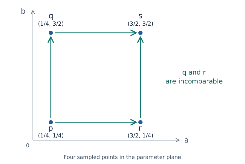
Arrows show comparisons among these four selected points. The comparison $p\leq s$ also holds and can be reached along either route. The diagram shows a finite sample of the parameter plane, not all of ℝ². Moving right or up increases a parameter; $q$ and $r$ have no order relation in either direction.
At each of these parameters we can compute a homology space. The specified inclusions give maps from the space at $p$ to those at $q$ and $r$, and from each of those spaces to the one at $s$. The parameter order supplies no structure map from $q$ to $r$ or from $r$ to $q$. This does not assert that no linear map could be written between their spaces; it says that neither direction is one of the comparisons prescribed by this module.
The ring was controlled by one real number, so every two parameter values could be ordered. With two coordinates we now have several directions of continuation, and these directions must agree wherever they meet.
A poset records the comparisons
A partially ordered set, or poset, is a set $Q$ together with a relation $\leq$ satisfying three rules. Each $q$ satisfies $q\leq q$ (reflexivity). If $q\leq r$ and $r\leq q$, then $q=r$ (antisymmetry). If $q\leq r$ and $r\leq s$, then $q\leq s$ (transitivity). These rules describe a consistent order without requiring that every pair be comparable.
The real line with its usual order is a poset in which every pair can be compared, also called a total order. The coordinatewise order on ℝ² is a partial order that is not total. A finite chain or the four selected points above, with their inherited comparisons, is also a poset. The same language can therefore describe one-parameter persistence, several parameters, and finite sets of comparisons.
The elements of $Q$ are parameters or labels; they are not the points of the shape $X_q$. For example, $(a,b)$ is a pair of thresholds specifying a shape, not a location inside that shape.
The spaces and maps must fit together
Fix a poset $Q$ and one coefficient field $\mathbb{k}$. A persistence module over $Q$, also called a $Q$-module or a representation of $Q$, consists of a vector space $M(q)$ for each $q\in Q$ and a linear map $M(q\leq r):M(q)\to M(r)$ for each comparison $q\leq r$. The space $M(q)$ is often called the stalk at $q$.
These data satisfy two compatibility rules:
\[M(q\leq q)=\operatorname{id}_{M(q)}, \qquad M(q\leq s)=M(r\leq s)\circ M(q\leq r) \quad\text{for }q\leq r\leq s.\]
The first rule says that staying at a parameter leaves its vectors unchanged. The second says that following a vector through an intermediate parameter gives the same result as taking the direct map. Composition is read from right to left: first use $M(q\leq r)$, then $M(r\leq s)$.
For the four points in the figure, this requires
\[M(q\leq s)\circ M(p\leq q) =M(p\leq s) =M(r\leq s)\circ M(p\leq r).\]
Thus the two routes from $M(p)$ to $M(s)$ must give the same linear map. This is what it means to say that the square commutes. Choosing a matrix for each drawn arrow is not enough: the two matrix products must agree. The omitted direct map is determined by either product.
For a filtration, this agreement comes from the inclusions of shapes: both routes include $X_p$ into the same $X_s$, and homology respects their composition. The abstract definition also allows modules to be specified directly by spaces and compatible maps, without first constructing shapes. In categorical language, it says that $M$ is a functor from the poset to vector spaces. Ezra Miller gives this formulation and the filtration construction in Definition 2.1 and Example 2.3 of Homological algebra of modules over posets.
All stalks use the same coefficient field. The field supplies the scalars inside a stalk; it is a separate choice from the parameter domain. A module can be indexed by real pairs while its vector spaces are over F₂ or ℚ. In the examples here the stalks are finite dimensional, although the poset indexing them can be infinite.
Figure placeholder: compare two routes around a square. Four selected comparable parameters will be linked to their stalks and structure matrices. Following a vector along either two-step route will show why the two compositions agree, making the compatibility equation visible.
Equal dimensions can hide different behavior
Even on two ordered parameters $u<v$, the dimensions do not determine the module. Over the same field, consider
\[A:\quad \mathbb{k}\xrightarrow{[1]}\mathbb{k}, \qquad B:\quad \mathbb{k}\xrightarrow{[0]}\mathbb{k}.\]
Each module has dimension one at both $u$ and $v$. In $A$, a nonzero vector at $u$ continues to a nonzero vector at $v$. In $B$, every vector from $u$ maps to zero; the nonzero vectors at $v$ are not inherited from $u$.
The rank of a map is the dimension of its image: how many independent vectors reach the target. The displayed map has rank one in $A$ and rank zero in $B$. Changing bases cannot turn a zero map into an identity map, so these are different modules even after allowing changes of coordinates in their stalks. A dimension plot would look identical for both.
This loss of information already occurs with one parameter. An ordinary barcode avoids it by recording continuation as well as dimensions: on this two-point poset, $A$ has one interval covering both points, whereas $B$ has two singleton intervals. With several parameters, arbitrary modules do not have an interval decomposition that plays the same general role as the ordinary barcode. The vector spaces and their compatible maps remain the object we need to retain; the broader distinction is discussed in Ezra Miller's account of bar codes and their extensions.
As a small check, return to the ring and compare the map from parameter 1 to parameter 4 with the map from 1 to 5. Their ranks are one and zero, respectively. The first preserves the loop class; the second kills it. Then return to $q=(1/4,3/2)$ and $r=(3/2,1/4)$. Asking for the rank of “the structure map from $q$ to $r$” is not a valid query: that comparison does not exist in the coordinatewise order.
How can we keep this object in finite form?
We now know what must be retained: a space at each parameter and a compatible map for each comparison. Over ℝ², that is an infinite collection. A dimension heatmap would omit the maps; a single increasing path would inspect only some of the parameters and comparisons.
The next question is when we can describe all of this with finitely many spaces and maps, together with a rule telling us which part of that finite description applies at an original parameter. That is the purpose of a finite encoding. Such a description requires hypotheses on the module; it is not available for every arbitrary assignment satisfying the module axioms.
The finite filtrations used here supply the needed finiteness through their construction.
Continue with finite encodings, where a module supported on the closed square $[0,2]^2$ supplies the next worked example. There we can check exactly how a finite model recovers both its spaces and its structure maps.